matrixStats.benchmarks
madDiff() benchmarks
This report benchmark the performance of madDiff() against alternative methods.
Alternative methods
- N/A
Data type “integer”
Data
> rvector <- function(n, mode = c("logical", "double", "integer"), range = c(-100, +100), na_prob = 0) {
+     mode <- match.arg(mode)
+     if (mode == "logical") {
+         x <- sample(c(FALSE, TRUE), size = n, replace = TRUE)
+     }     else {
+         x <- runif(n, min = range[1], max = range[2])
+     }
+     storage.mode(x) <- mode
+     if (na_prob > 0)
+         x[sample(n, size = na_prob * n)] <- NA
+     x
+ }
> rvectors <- function(scale = 10, seed = 1, ...) {
+     set.seed(seed)
+     data <- list()
+     data[[1]] <- rvector(n = scale * 100, ...)
+     data[[2]] <- rvector(n = scale * 1000, ...)
+     data[[3]] <- rvector(n = scale * 10000, ...)
+     data[[4]] <- rvector(n = scale * 1e+05, ...)
+     data[[5]] <- rvector(n = scale * 1e+06, ...)
+     names(data) <- sprintf("n = %d", sapply(data, FUN = length))
+     data
+ }
> data <- rvectors(mode = mode)
> data <- data[1:4]
Results
n = 1000 vector
All elements
> x <- data[["n = 1000"]]
> stats <- microbenchmark(madDiff = madDiff(x), mad = mad(x), diff = diff(x), unit = "ms")
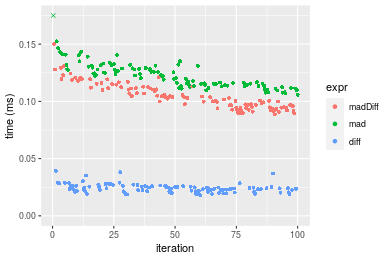
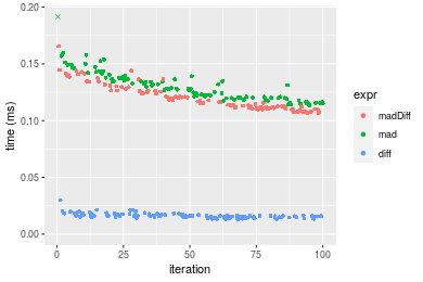
Table: Benchmarking of madDiff(), mad() and diff() on integer+n = 1000 data. The top panel shows times in milliseconds and the bottom panel shows relative times.
| expr | min | lq | mean | median | uq | max | |
|---|---|---|---|---|---|---|---|
| 3 | diff | 0.017752 | 0.0214995 | 0.0241288 | 0.023748 | 0.0259275 | 0.039277 |
| 1 | madDiff | 0.088629 | 0.0949025 | 0.1046152 | 0.103037 | 0.1121460 | 0.150218 |
| 2 | mad | 0.105680 | 0.1136725 | 0.1237513 | 0.122174 | 0.1292590 | 0.270952 |
| expr | min | lq | mean | median | uq | max | |
|---|---|---|---|---|---|---|---|
| 3 | diff | 1.000000 | 1.000000 | 1.000000 | 1.000000 | 1.000000 | 1.000000 |
| 1 | madDiff | 4.992621 | 4.414172 | 4.335696 | 4.338765 | 4.325369 | 3.824579 |
| 2 | mad | 5.953132 | 5.287216 | 5.128775 | 5.144602 | 4.985402 | 6.898490 |
Figure: Benchmarking of madDiff(), mad() and diff() on integer+n = 1000 data. Outliers are displayed as crosses. Times are in milliseconds.
n = 10000 vector
All elements
> x <- data[["n = 10000"]]
> stats <- microbenchmark(madDiff = madDiff(x), mad = mad(x), diff = diff(x), unit = "ms")
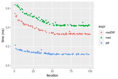
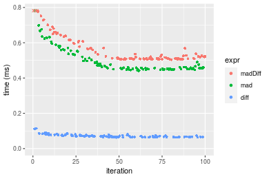
Table: Benchmarking of madDiff(), mad() and diff() on integer+n = 10000 data. The top panel shows times in milliseconds and the bottom panel shows relative times.
| expr | min | lq | mean | median | uq | max | |
|---|---|---|---|---|---|---|---|
| 3 | diff | 0.113027 | 0.1183590 | 0.1317600 | 0.1249735 | 0.1411005 | 0.213902 |
| 1 | madDiff | 0.324380 | 0.3301435 | 0.3712612 | 0.3364710 | 0.4056640 | 0.638642 |
| 2 | mad | 0.411193 | 0.4192715 | 0.4678962 | 0.4313300 | 0.5069095 | 0.680386 |
| expr | min | lq | mean | median | uq | max | |
|---|---|---|---|---|---|---|---|
| 3 | diff | 1.000000 | 1.000000 | 1.000000 | 1.000000 | 1.000000 | 1.000000 |
| 1 | madDiff | 2.869934 | 2.789340 | 2.817708 | 2.692339 | 2.875000 | 2.985676 |
| 2 | mad | 3.638007 | 3.542371 | 3.551125 | 3.451372 | 3.592542 | 3.180830 |
Figure: Benchmarking of madDiff(), mad() and diff() on integer+n = 10000 data. Outliers are displayed as crosses. Times are in milliseconds.
n = 100000 vector
All elements
> x <- data[["n = 100000"]]
> stats <- microbenchmark(madDiff = madDiff(x), mad = mad(x), diff = diff(x), unit = "ms")
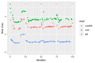
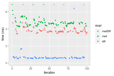
Table: Benchmarking of madDiff(), mad() and diff() on integer+n = 100000 data. The top panel shows times in milliseconds and the bottom panel shows relative times.
| expr | min | lq | mean | median | uq | max | |
|---|---|---|---|---|---|---|---|
| 3 | diff | 1.036132 | 1.130519 | 1.300537 | 1.172840 | 1.255360 | 7.771759 |
| 1 | madDiff | 2.575734 | 2.813886 | 3.053933 | 2.850616 | 2.926643 | 9.541398 |
| 2 | mad | 3.337370 | 3.567168 | 3.835025 | 3.658603 | 3.796289 | 10.060741 |
| expr | min | lq | mean | median | uq | max | |
|---|---|---|---|---|---|---|---|
| 3 | diff | 1.000000 | 1.000000 | 1.000000 | 1.000000 | 1.000000 | 1.000000 |
| 1 | madDiff | 2.485913 | 2.489021 | 2.348209 | 2.430524 | 2.331318 | 1.227701 |
| 2 | mad | 3.220989 | 3.155337 | 2.948801 | 3.119440 | 3.024064 | 1.294526 |
Figure: Benchmarking of madDiff(), mad() and diff() on integer+n = 100000 data. Outliers are displayed as crosses. Times are in milliseconds.
n = 1000000 vector
All elements
> x <- data[["n = 1000000"]]
> stats <- microbenchmark(madDiff = madDiff(x), mad = mad(x), diff = diff(x), unit = "ms")
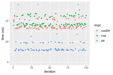
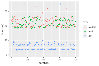
Table: Benchmarking of madDiff(), mad() and diff() on integer+n = 1000000 data. The top panel shows times in milliseconds and the bottom panel shows relative times.
| expr | min | lq | mean | median | uq | max | |
|---|---|---|---|---|---|---|---|
| 3 | diff | 11.02840 | 11.65005 | 17.75196 | 12.08700 | 18.66433 | 392.88244 |
| 1 | madDiff | 31.70395 | 33.02597 | 36.01248 | 34.33064 | 40.07227 | 50.52308 |
| 2 | mad | 34.74192 | 36.15372 | 39.83439 | 37.17157 | 44.77725 | 58.22014 |
| expr | min | lq | mean | median | uq | max | |
|---|---|---|---|---|---|---|---|
| 3 | diff | 1.000000 | 1.000000 | 1.000000 | 1.000000 | 1.000000 | 1.0000000 |
| 1 | madDiff | 2.874754 | 2.834836 | 2.028647 | 2.840294 | 2.146998 | 0.1285959 |
| 2 | mad | 3.150222 | 3.103311 | 2.243943 | 3.075334 | 2.399082 | 0.1481872 |
Figure: Benchmarking of madDiff(), mad() and diff() on integer+n = 1000000 data. Outliers are displayed as crosses. Times are in milliseconds.
Data type “double”
Data
> rvector <- function(n, mode = c("logical", "double", "integer"), range = c(-100, +100), na_prob = 0) {
+     mode <- match.arg(mode)
+     if (mode == "logical") {
+         x <- sample(c(FALSE, TRUE), size = n, replace = TRUE)
+     }     else {
+         x <- runif(n, min = range[1], max = range[2])
+     }
+     storage.mode(x) <- mode
+     if (na_prob > 0)
+         x[sample(n, size = na_prob * n)] <- NA
+     x
+ }
> rvectors <- function(scale = 10, seed = 1, ...) {
+     set.seed(seed)
+     data <- list()
+     data[[1]] <- rvector(n = scale * 100, ...)
+     data[[2]] <- rvector(n = scale * 1000, ...)
+     data[[3]] <- rvector(n = scale * 10000, ...)
+     data[[4]] <- rvector(n = scale * 1e+05, ...)
+     data[[5]] <- rvector(n = scale * 1e+06, ...)
+     names(data) <- sprintf("n = %d", sapply(data, FUN = length))
+     data
+ }
> data <- rvectors(mode = mode)
> data <- data[1:4]
Results
n = 1000 vector
All elements
> x <- data[["n = 1000"]]
> stats <- microbenchmark(madDiff = madDiff(x), mad = mad(x), diff = diff(x), unit = "ms")
Table: Benchmarking of madDiff(), mad() and diff() on double+n = 1000 data. The top panel shows times in milliseconds and the bottom panel shows relative times.
| expr | min | lq | mean | median | uq | max | |
|---|---|---|---|---|---|---|---|
| 3 | diff | 0.013201 | 0.0147700 | 0.0162467 | 0.0159435 | 0.016973 | 0.029938 |
| 1 | madDiff | 0.106338 | 0.1109705 | 0.1200912 | 0.1163020 | 0.126430 | 0.165608 |
| 2 | mad | 0.113455 | 0.1201745 | 0.1314006 | 0.1279825 | 0.137668 | 0.270726 |
| expr | min | lq | mean | median | uq | max | |
|---|---|---|---|---|---|---|---|
| 3 | diff | 1.000000 | 1.000000 | 1.000000 | 1.000000 | 1.000000 | 1.000000 |
| 1 | madDiff | 8.055299 | 7.513236 | 7.391731 | 7.294634 | 7.448889 | 5.531699 |
| 2 | mad | 8.594425 | 8.136391 | 8.087838 | 8.027252 | 8.111000 | 9.042889 |
Figure: Benchmarking of madDiff(), mad() and diff() on double+n = 1000 data. Outliers are displayed as crosses. Times are in milliseconds.
n = 10000 vector
All elements
> x <- data[["n = 10000"]]
> stats <- microbenchmark(madDiff = madDiff(x), mad = mad(x), diff = diff(x), unit = "ms")
Table: Benchmarking of madDiff(), mad() and diff() on double+n = 10000 data. The top panel shows times in milliseconds and the bottom panel shows relative times.
| expr | min | lq | mean | median | uq | max | |
|---|---|---|---|---|---|---|---|
| 3 | diff | 0.063052 | 0.0658795 | 0.0720300 | 0.0700025 | 0.0759765 | 0.114779 |
| 2 | mad | 0.441619 | 0.4511230 | 0.4968053 | 0.4611525 | 0.5256760 | 0.782934 |
| 1 | madDiff | 0.504355 | 0.5091125 | 0.5690519 | 0.5213725 | 0.6086355 | 0.936383 |
| expr | min | lq | mean | median | uq | max | |
|---|---|---|---|---|---|---|---|
| 3 | diff | 1.000000 | 1.000000 | 1.000000 | 1.000000 | 1.000000 | 1.000000 |
| 2 | mad | 7.004044 | 6.847699 | 6.897198 | 6.587658 | 6.918929 | 6.821230 |
| 1 | madDiff | 7.999033 | 7.727935 | 7.900204 | 7.447913 | 8.010839 | 8.158139 |
Figure: Benchmarking of madDiff(), mad() and diff() on double+n = 10000 data. Outliers are displayed as crosses. Times are in milliseconds.
n = 100000 vector
All elements
> x <- data[["n = 100000"]]
> stats <- microbenchmark(madDiff = madDiff(x), mad = mad(x), diff = diff(x), unit = "ms")
Table: Benchmarking of madDiff(), mad() and diff() on double+n = 100000 data. The top panel shows times in milliseconds and the bottom panel shows relative times.
| expr | min | lq | mean | median | uq | max | |
|---|---|---|---|---|---|---|---|
| 3 | diff | 0.519885 | 0.570392 | 0.6985906 | 0.6014705 | 0.651661 | 6.399512 |
| 1 | madDiff | 3.394157 | 3.652373 | 4.0606775 | 3.7422355 | 3.987932 | 10.796630 |
| 2 | mad | 4.276920 | 4.456988 | 4.8640088 | 4.6598885 | 4.834231 | 11.028984 |
| expr | min | lq | mean | median | uq | max | |
|---|---|---|---|---|---|---|---|
| 3 | diff | 1.000000 | 1.000000 | 1.000000 | 1.000000 | 1.000000 | 1.000000 |
| 1 | madDiff | 6.528669 | 6.403268 | 5.812671 | 6.221811 | 6.119643 | 1.687102 |
| 2 | mad | 8.226665 | 7.813903 | 6.962603 | 7.747493 | 7.418322 | 1.723410 |
Figure: Benchmarking of madDiff(), mad() and diff() on double+n = 100000 data. Outliers are displayed as crosses. Times are in milliseconds.
n = 1000000 vector
All elements
> x <- data[["n = 1000000"]]
> stats <- microbenchmark(madDiff = madDiff(x), mad = mad(x), diff = diff(x), unit = "ms")
Table: Benchmarking of madDiff(), mad() and diff() on double+n = 1000000 data. The top panel shows times in milliseconds and the bottom panel shows relative times.
| expr | min | lq | mean | median | uq | max | |
|---|---|---|---|---|---|---|---|
| 3 | diff | 6.691625 | 7.436153 | 14.86925 | 8.213351 | 14.24587 | 388.54273 |
| 2 | mad | 36.656780 | 39.197105 | 43.52137 | 42.272902 | 47.81036 | 53.08252 |
| 1 | madDiff | 37.511064 | 39.747759 | 48.87698 | 44.476872 | 49.17636 | 426.27070 |
| expr | min | lq | mean | median | uq | max | |
|---|---|---|---|---|---|---|---|
| 3 | diff | 1.000000 | 1.000000 | 1.000000 | 1.000000 | 1.000000 | 1.0000000 |
| 2 | mad | 5.478009 | 5.271154 | 2.926939 | 5.146852 | 3.356086 | 0.1366195 |
| 1 | madDiff | 5.605673 | 5.345205 | 3.287119 | 5.415192 | 3.451974 | 1.0971012 |
Figure: Benchmarking of madDiff(), mad() and diff() on double+n = 1000000 data. Outliers are displayed as crosses. Times are in milliseconds.
Appendix
Session information
R version 4.1.1 Patched (2021-08-10 r80727)
Platform: x86_64-pc-linux-gnu (64-bit)
Running under: Ubuntu 18.04.5 LTS

Matrix products: default
BLAS:   /home/hb/software/R-devel/R-4-1-branch/lib/R/lib/libRblas.so
LAPACK: /home/hb/software/R-devel/R-4-1-branch/lib/R/lib/libRlapack.so

locale:
 [1] LC_CTYPE=en_US.UTF-8       LC_NUMERIC=C
 [3] LC_TIME=en_US.UTF-8        LC_COLLATE=en_US.UTF-8
 [5] LC_MONETARY=en_US.UTF-8    LC_MESSAGES=en_US.UTF-8
 [7] LC_PAPER=en_US.UTF-8       LC_NAME=C
 [9] LC_ADDRESS=C               LC_TELEPHONE=C
[11] LC_MEASUREMENT=en_US.UTF-8 LC_IDENTIFICATION=C

attached base packages:
[1] stats     graphics  grDevices utils     datasets  methods   base

other attached packages:
[1] microbenchmark_1.4-7   matrixStats_0.60.1     ggplot2_3.3.5
[4] knitr_1.33             R.devices_2.17.0       R.utils_2.10.1
[7] R.oo_1.24.0            R.methodsS3_1.8.1-9001 history_0.0.1-9000

loaded via a namespace (and not attached):
 [1] Biobase_2.52.0          httr_1.4.2              splines_4.1.1
 [4] bit64_4.0.5             network_1.17.1          assertthat_0.2.1
 [7] highr_0.9               stats4_4.1.1            blob_1.2.2
[10] GenomeInfoDbData_1.2.6  robustbase_0.93-8       pillar_1.6.2
[13] RSQLite_2.2.8           lattice_0.20-44         glue_1.4.2
[16] digest_0.6.27           XVector_0.32.0          colorspace_2.0-2
[19] Matrix_1.3-4            XML_3.99-0.7            pkgconfig_2.0.3
[22] zlibbioc_1.38.0         genefilter_1.74.0       purrr_0.3.4
[25] ergm_4.1.2              xtable_1.8-4            scales_1.1.1
[28] tibble_3.1.4            annotate_1.70.0         KEGGREST_1.32.0
[31] farver_2.1.0            generics_0.1.0          IRanges_2.26.0
[34] ellipsis_0.3.2          cachem_1.0.6            withr_2.4.2
[37] BiocGenerics_0.38.0     mime_0.11               survival_3.2-13
[40] magrittr_2.0.1          crayon_1.4.1            statnet.common_4.5.0
[43] memoise_2.0.0           laeken_0.5.1            fansi_0.5.0
[46] R.cache_0.15.0          MASS_7.3-54             R.rsp_0.44.0
[49] progressr_0.8.0         tools_4.1.1             lifecycle_1.0.0
[52] S4Vectors_0.30.0        trust_0.1-8             munsell_0.5.0
[55] tabby_0.0.1-9001        AnnotationDbi_1.54.1    Biostrings_2.60.2
[58] compiler_4.1.1          GenomeInfoDb_1.28.1     rlang_0.4.11
[61] grid_4.1.1              RCurl_1.98-1.4          cwhmisc_6.6
[64] rappdirs_0.3.3          startup_0.15.0          labeling_0.4.2
[67] bitops_1.0-7            base64enc_0.1-3         boot_1.3-28
[70] gtable_0.3.0            DBI_1.1.1               markdown_1.1
[73] R6_2.5.1                lpSolveAPI_5.5.2.0-17.7 rle_0.9.2
[76] dplyr_1.0.7             fastmap_1.1.0           bit_4.0.4
[79] utf8_1.2.2              parallel_4.1.1          Rcpp_1.0.7
[82] vctrs_0.3.8             png_0.1-7               DEoptimR_1.0-9
[85] tidyselect_1.1.1        xfun_0.25               coda_0.19-4
Total processing time was 29.99 secs.
Reproducibility
To reproduce this report, do:
html <- matrixStats:::benchmark('madDiff')
Copyright Henrik Bengtsson. Last updated on 2021-08-25 19:20:20 (+0200 UTC). Powered by RSP.