matrixStats.benchmarks
count() benchmarks on subsetted computation
This report benchmark the performance of count() on subsetted computation.
Data type “integer”
Data
> rvector <- function(n, mode = c("logical", "double", "integer"), range = c(-100, +100), na_prob = 0) {
+     mode <- match.arg(mode)
+     if (mode == "logical") {
+         x <- sample(c(FALSE, TRUE), size = n, replace = TRUE)
+     }     else {
+         x <- runif(n, min = range[1], max = range[2])
+     }
+     storage.mode(x) <- mode
+     if (na_prob > 0)
+         x[sample(n, size = na_prob * n)] <- NA
+     x
+ }
> rvectors <- function(scale = 10, seed = 1, ...) {
+     set.seed(seed)
+     data <- list()
+     data[[1]] <- rvector(n = scale * 100, ...)
+     data[[2]] <- rvector(n = scale * 1000, ...)
+     data[[3]] <- rvector(n = scale * 10000, ...)
+     data[[4]] <- rvector(n = scale * 1e+05, ...)
+     data[[5]] <- rvector(n = scale * 1e+06, ...)
+     names(data) <- sprintf("n = %d", sapply(data, FUN = length))
+     data
+ }
> data <- rvectors(mode = mode)
Results
n = 1000 vector
> x <- data[["n = 1000"]]
> idxs <- sample.int(length(x), size = length(x) * 0.7)
> x_S <- x[idxs]
> gc()
           used  (Mb) gc trigger  (Mb) max used  (Mb)
Ncells  5337704 285.1    8529671 455.6  8529671 455.6
Vcells 16188595 123.6   31876688 243.2 60562128 462.1
> stats <- microbenchmark(count_x_S = count(x_S, value), `count(x, idxs)` = count(x, idxs = idxs, value),
+     `count(x[idxs])` = count(x[idxs], value), unit = "ms")
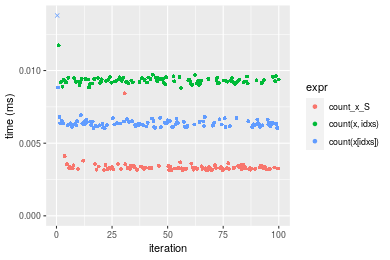
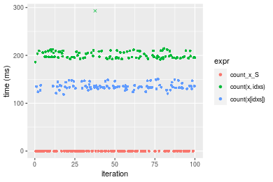
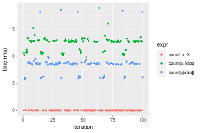
Table: Benchmarking of count_x_S(), count(x, idxs)() and count(x[idxs])() on integer+n = 1000 data. The top panel shows times in milliseconds and the bottom panel shows relative times.
| expr | min | lq | mean | median | uq | max | |
|---|---|---|---|---|---|---|---|
| 1 | count_x_S | 0.003124 | 0.0032290 | 0.0033736 | 0.0032875 | 0.003396 | 0.008437 |
| 3 | count(x[idxs]) | 0.006028 | 0.0062300 | 0.0083352 | 0.0063275 | 0.006489 | 0.201845 |
| 2 | count(x, idxs) | 0.008802 | 0.0091875 | 0.0093289 | 0.0093030 | 0.009424 | 0.011735 |
| expr | min | lq | mean | median | uq | max | |
|---|---|---|---|---|---|---|---|
| 1 | count_x_S | 1.000000 | 1.000000 | 1.000000 | 1.000000 | 1.000000 | 1.000000 |
| 3 | count(x[idxs]) | 1.929577 | 1.929390 | 2.470705 | 1.924715 | 1.910777 | 23.923788 |
| 2 | count(x, idxs) | 2.817542 | 2.845308 | 2.765271 | 2.829810 | 2.775029 | 1.390897 |
Figure: Benchmarking of count_x_S(), count(x, idxs)() and count(x[idxs])() on integer+n = 1000 data. Outliers are displayed as crosses. Times are in milliseconds.
n = 10000 vector
> x <- data[["n = 10000"]]
> idxs <- sample.int(length(x), size = length(x) * 0.7)
> x_S <- x[idxs]
> gc()
           used  (Mb) gc trigger  (Mb) max used  (Mb)
Ncells  5325873 284.5    8529671 455.6  8529671 455.6
Vcells 15826127 120.8   31876688 243.2 60562128 462.1
> stats <- microbenchmark(count_x_S = count(x_S, value), `count(x, idxs)` = count(x, idxs = idxs, value),
+     `count(x[idxs])` = count(x[idxs], value), unit = "ms")
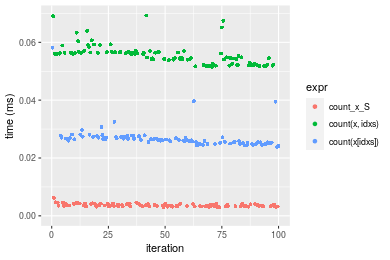
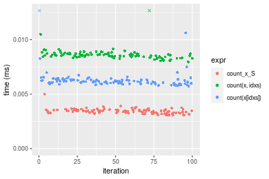
Table: Benchmarking of count_x_S(), count(x, idxs)() and count(x[idxs])() on integer+n = 10000 data. The top panel shows times in milliseconds and the bottom panel shows relative times.
| expr | min | lq | mean | median | uq | max | |
|---|---|---|---|---|---|---|---|
| 1 | count_x_S | 0.002959 | 0.0033245 | 0.0036661 | 0.003490 | 0.0040450 | 0.006257 |
| 3 | count(x[idxs]) | 0.023779 | 0.0252135 | 0.0268024 | 0.026144 | 0.0270715 | 0.058188 |
| 2 | count(x, idxs) | 0.051535 | 0.0539220 | 0.0557227 | 0.055899 | 0.0565915 | 0.069279 |
| expr | min | lq | mean | median | uq | max | |
|---|---|---|---|---|---|---|---|
| 1 | count_x_S | 1.000000 | 1.000000 | 1.000000 | 1.000000 | 1.000000 | 1.000000 |
| 3 | count(x[idxs]) | 8.036161 | 7.584148 | 7.310963 | 7.491117 | 6.692583 | 9.299664 |
| 2 | count(x, idxs) | 17.416357 | 16.219582 | 15.199612 | 16.016905 | 13.990482 | 11.072239 |
Figure: Benchmarking of count_x_S(), count(x, idxs)() and count(x[idxs])() on integer+n = 10000 data. Outliers are displayed as crosses. Times are in milliseconds.
n = 100000 vector
> x <- data[["n = 100000"]]
> idxs <- sample.int(length(x), size = length(x) * 0.7)
> x_S <- x[idxs]
> gc()
           used  (Mb) gc trigger  (Mb) max used  (Mb)
Ncells  5325945 284.5    8529671 455.6  8529671 455.6
Vcells 15889687 121.3   31876688 243.2 60562128 462.1
> stats <- microbenchmark(count_x_S = count(x_S, value), `count(x, idxs)` = count(x, idxs = idxs, value),
+     `count(x[idxs])` = count(x[idxs], value), unit = "ms")
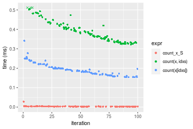
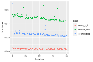
Table: Benchmarking of count_x_S(), count(x, idxs)() and count(x[idxs])() on integer+n = 100000 data. The top panel shows times in milliseconds and the bottom panel shows relative times.
| expr | min | lq | mean | median | uq | max | |
|---|---|---|---|---|---|---|---|
| 1 | count_x_S | 0.001966 | 0.002521 | 0.0033355 | 0.0030575 | 0.003545 | 0.027890 |
| 3 | count(x[idxs]) | 0.154013 | 0.171140 | 0.1946933 | 0.1920005 | 0.209566 | 0.341173 |
| 2 | count(x, idxs) | 0.322152 | 0.340729 | 0.3890901 | 0.3765425 | 0.422771 | 0.526677 |
| expr | min | lq | mean | median | uq | max | |
|---|---|---|---|---|---|---|---|
| 1 | count_x_S | 1.00000 | 1.00000 | 1.00000 | 1.00000 | 1.00000 | 1.00000 |
| 3 | count(x[idxs]) | 78.33825 | 67.88576 | 58.37075 | 62.79657 | 59.11594 | 12.23281 |
| 2 | count(x, idxs) | 163.86165 | 135.15629 | 116.65260 | 123.15372 | 119.25839 | 18.88408 |
Figure: Benchmarking of count_x_S(), count(x, idxs)() and count(x[idxs])() on integer+n = 100000 data. Outliers are displayed as crosses. Times are in milliseconds.
n = 1000000 vector
> x <- data[["n = 1000000"]]
> idxs <- sample.int(length(x), size = length(x) * 0.7)
> x_S <- x[idxs]
> gc()
           used  (Mb) gc trigger  (Mb) max used  (Mb)
Ncells  5326017 284.5    8529671 455.6  8529671 455.6
Vcells 16519736 126.1   31876688 243.2 60562128 462.1
> stats <- microbenchmark(count_x_S = count(x_S, value), `count(x, idxs)` = count(x, idxs = idxs, value),
+     `count(x[idxs])` = count(x[idxs], value), unit = "ms")
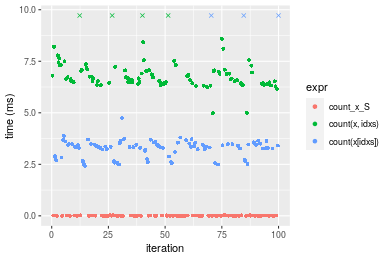
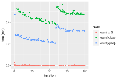
Table: Benchmarking of count_x_S(), count(x, idxs)() and count(x[idxs])() on integer+n = 1000000 data. The top panel shows times in milliseconds and the bottom panel shows relative times.
| expr | min | lq | mean | median | uq | max | |
|---|---|---|---|---|---|---|---|
| 1 | count_x_S | 0.002259 | 0.002726 | 0.0087498 | 0.004727 | 0.016404 | 0.029541 |
| 3 | count(x[idxs]) | 2.430345 | 3.218565 | 3.5464096 | 3.356628 | 3.504419 | 12.517851 |
| 2 | count(x, idxs) | 4.987628 | 6.450848 | 7.0870798 | 6.666243 | 7.080705 | 14.853591 |
| expr | min | lq | mean | median | uq | max | |
|---|---|---|---|---|---|---|---|
| 1 | count_x_S | 1.000 | 1.000 | 1.0000 | 1.000 | 1.000 | 1.0000 |
| 3 | count(x[idxs]) | 1075.850 | 1180.691 | 405.3151 | 710.097 | 213.632 | 423.7450 |
| 2 | count(x, idxs) | 2207.892 | 2366.415 | 809.9742 | 1410.248 | 431.645 | 502.8127 |
Figure: Benchmarking of count_x_S(), count(x, idxs)() and count(x[idxs])() on integer+n = 1000000 data. Outliers are displayed as crosses. Times are in milliseconds.
n = 10000000 vector
> x <- data[["n = 10000000"]]
> idxs <- sample.int(length(x), size = length(x) * 0.7)
> x_S <- x[idxs]
> gc()
           used  (Mb) gc trigger  (Mb) max used  (Mb)
Ncells  5326089 284.5    8529671 455.6  8529671 455.6
Vcells 22819784 174.2   38332025 292.5 60562128 462.1
> stats <- microbenchmark(count_x_S = count(x_S, value), `count(x, idxs)` = count(x, idxs = idxs, value),
+     `count(x[idxs])` = count(x[idxs], value), unit = "ms")
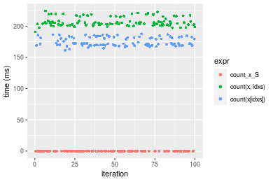
Table: Benchmarking of count_x_S(), count(x, idxs)() and count(x[idxs])() on integer+n = 10000000 data. The top panel shows times in milliseconds and the bottom panel shows relative times.
| expr | min | lq | mean | median | uq | max | |
|---|---|---|---|---|---|---|---|
| 1 | count_x_S | 0.004811 | 0.0084275 | 0.0226571 | 0.011918 | 0.0398745 | 0.060674 |
| 3 | count(x[idxs]) | 118.524917 | 131.7575515 | 135.2031126 | 133.612279 | 137.3446095 | 150.740488 |
| 2 | count(x, idxs) | 186.045876 | 195.3748840 | 204.4757756 | 197.859924 | 208.1215880 | 570.309314 |
| expr | min | lq | mean | median | uq | max | |
|---|---|---|---|---|---|---|---|
| 1 | count_x_S | 1.00 | 1.00 | 1.000 | 1.00 | 1.000 | 1.000 |
| 3 | count(x[idxs]) | 24636.23 | 15634.24 | 5967.359 | 11210.96 | 3444.422 | 2484.433 |
| 2 | count(x, idxs) | 38670.94 | 23183.02 | 9024.795 | 16601.77 | 5219.416 | 9399.567 |
Figure: Benchmarking of count_x_S(), count(x, idxs)() and count(x[idxs])() on integer+n = 10000000 data. Outliers are displayed as crosses. Times are in milliseconds.
Data type “double”
Data
> rvector <- function(n, mode = c("logical", "double", "integer"), range = c(-100, +100), na_prob = 0) {
+     mode <- match.arg(mode)
+     if (mode == "logical") {
+         x <- sample(c(FALSE, TRUE), size = n, replace = TRUE)
+     }     else {
+         x <- runif(n, min = range[1], max = range[2])
+     }
+     storage.mode(x) <- mode
+     if (na_prob > 0)
+         x[sample(n, size = na_prob * n)] <- NA
+     x
+ }
> rvectors <- function(scale = 10, seed = 1, ...) {
+     set.seed(seed)
+     data <- list()
+     data[[1]] <- rvector(n = scale * 100, ...)
+     data[[2]] <- rvector(n = scale * 1000, ...)
+     data[[3]] <- rvector(n = scale * 10000, ...)
+     data[[4]] <- rvector(n = scale * 1e+05, ...)
+     data[[5]] <- rvector(n = scale * 1e+06, ...)
+     names(data) <- sprintf("n = %d", sapply(data, FUN = length))
+     data
+ }
> data <- rvectors(mode = mode)
Results
n = 1000 vector
> x <- data[["n = 1000"]]
> idxs <- sample.int(length(x), size = length(x) * 0.7)
> x_S <- x[idxs]
> gc()
           used  (Mb) gc trigger  (Mb) max used  (Mb)
Ncells  5326164 284.5    8529671 455.6  8529671 455.6
Vcells 21376985 163.1   46078430 351.6 60562128 462.1
> stats <- microbenchmark(count_x_S = count(x_S, value), `count(x, idxs)` = count(x, idxs = idxs, value),
+     `count(x[idxs])` = count(x[idxs], value), unit = "ms")
Table: Benchmarking of count_x_S(), count(x, idxs)() and count(x[idxs])() on double+n = 1000 data. The top panel shows times in milliseconds and the bottom panel shows relative times.
| expr | min | lq | mean | median | uq | max | |
|---|---|---|---|---|---|---|---|
| 1 | count_x_S | 0.003063 | 0.0032870 | 0.0034310 | 0.0034255 | 0.0035500 | 0.005006 |
| 3 | count(x[idxs]) | 0.005732 | 0.0060000 | 0.0065527 | 0.0061685 | 0.0063315 | 0.036603 |
| 2 | count(x, idxs) | 0.007954 | 0.0084305 | 0.0087315 | 0.0085650 | 0.0087110 | 0.022903 |
| expr | min | lq | mean | median | uq | max | |
|---|---|---|---|---|---|---|---|
| 1 | count_x_S | 1.000000 | 1.000000 | 1.000000 | 1.000000 | 1.000000 | 1.000000 |
| 3 | count(x[idxs]) | 1.871368 | 1.825373 | 1.909826 | 1.800759 | 1.783521 | 7.311826 |
| 2 | count(x, idxs) | 2.596801 | 2.564801 | 2.544870 | 2.500365 | 2.453803 | 4.575110 |
Figure: Benchmarking of count_x_S(), count(x, idxs)() and count(x[idxs])() on double+n = 1000 data. Outliers are displayed as crosses. Times are in milliseconds.
n = 10000 vector
> x <- data[["n = 10000"]]
> idxs <- sample.int(length(x), size = length(x) * 0.7)
> x_S <- x[idxs]
> gc()
           used  (Mb) gc trigger  (Mb) max used  (Mb)
Ncells  5326233 284.5    8529671 455.6  8529671 455.6
Vcells 21386477 163.2   46078430 351.6 60562128 462.1
> stats <- microbenchmark(count_x_S = count(x_S, value), `count(x, idxs)` = count(x, idxs = idxs, value),
+     `count(x[idxs])` = count(x[idxs], value), unit = "ms")
Table: Benchmarking of count_x_S(), count(x, idxs)() and count(x[idxs])() on double+n = 10000 data. The top panel shows times in milliseconds and the bottom panel shows relative times.
| expr | min | lq | mean | median | uq | max | |
|---|---|---|---|---|---|---|---|
| 1 | count_x_S | 0.003036 | 0.0033195 | 0.0036829 | 0.0035275 | 0.0040255 | 0.006112 |
| 3 | count(x[idxs]) | 0.021808 | 0.0233370 | 0.0252238 | 0.0247295 | 0.0254530 | 0.076580 |
| 2 | count(x, idxs) | 0.043698 | 0.0460250 | 0.0486790 | 0.0483470 | 0.0503150 | 0.066311 |
| expr | min | lq | mean | median | uq | max | |
|---|---|---|---|---|---|---|---|
| 1 | count_x_S | 1.000000 | 1.000000 | 1.000000 | 1.000000 | 1.000000 | 1.00000 |
| 3 | count(x[idxs]) | 7.183136 | 7.030276 | 6.848862 | 7.010489 | 6.322941 | 12.52945 |
| 2 | count(x, idxs) | 14.393281 | 13.865040 | 13.217504 | 13.705741 | 12.499068 | 10.84931 |
Figure: Benchmarking of count_x_S(), count(x, idxs)() and count(x[idxs])() on double+n = 10000 data. Outliers are displayed as crosses. Times are in milliseconds.
n = 100000 vector
> x <- data[["n = 100000"]]
> idxs <- sample.int(length(x), size = length(x) * 0.7)
> x_S <- x[idxs]
> gc()
           used  (Mb) gc trigger  (Mb) max used  (Mb)
Ncells  5326305 284.5    8529671 455.6  8529671 455.6
Vcells 21481355 163.9   46078430 351.6 60562128 462.1
> stats <- microbenchmark(count_x_S = count(x_S, value), `count(x, idxs)` = count(x, idxs = idxs, value),
+     `count(x[idxs])` = count(x[idxs], value), unit = "ms")
Table: Benchmarking of count_x_S(), count(x, idxs)() and count(x[idxs])() on double+n = 100000 data. The top panel shows times in milliseconds and the bottom panel shows relative times.
| expr | min | lq | mean | median | uq | max | |
|---|---|---|---|---|---|---|---|
| 1 | count_x_S | 0.001986 | 0.0025905 | 0.0033840 | 0.0031240 | 0.0035645 | 0.028566 |
| 3 | count(x[idxs]) | 0.206053 | 0.2353825 | 0.2762238 | 0.2576055 | 0.3195455 | 0.471001 |
| 2 | count(x, idxs) | 0.380342 | 0.4334860 | 0.4658087 | 0.4761000 | 0.4900790 | 0.561349 |
| expr | min | lq | mean | median | uq | max | |
|---|---|---|---|---|---|---|---|
| 1 | count_x_S | 1.0000 | 1.00000 | 1.00000 | 1.00000 | 1.00000 | 1.00000 |
| 3 | count(x[idxs]) | 103.7528 | 90.86373 | 81.62617 | 82.46015 | 89.64665 | 16.48817 |
| 2 | count(x, idxs) | 191.5116 | 167.33681 | 137.64991 | 152.40077 | 137.48885 | 19.65095 |
Figure: Benchmarking of count_x_S(), count(x, idxs)() and count(x[idxs])() on double+n = 100000 data. Outliers are displayed as crosses. Times are in milliseconds.
n = 1000000 vector
> x <- data[["n = 1000000"]]
> idxs <- sample.int(length(x), size = length(x) * 0.7)
> x_S <- x[idxs]
> gc()
           used  (Mb) gc trigger  (Mb) max used  (Mb)
Ncells  5326377 284.5    8529671 455.6  8529671 455.6
Vcells 22426799 171.2   46078430 351.6 60562128 462.1
> stats <- microbenchmark(count_x_S = count(x_S, value), `count(x, idxs)` = count(x, idxs = idxs, value),
+     `count(x[idxs])` = count(x[idxs], value), unit = "ms")
Table: Benchmarking of count_x_S(), count(x, idxs)() and count(x[idxs])() on double+n = 1000000 data. The top panel shows times in milliseconds and the bottom panel shows relative times.
| expr | min | lq | mean | median | uq | max | |
|---|---|---|---|---|---|---|---|
| 1 | count_x_S | 0.003225 | 0.003772 | 0.010707 | 0.006211 | 0.020316 | 0.030798 |
| 3 | count(x[idxs]) | 5.751479 | 8.461458 | 8.665678 | 8.584268 | 8.747654 | 18.502944 |
| 2 | count(x, idxs) | 10.133536 | 12.543808 | 12.468542 | 12.700802 | 12.899890 | 22.428013 |
| expr | min | lq | mean | median | uq | max | |
|---|---|---|---|---|---|---|---|
| 1 | count_x_S | 1.000 | 1.000 | 1.0000 | 1.000 | 1.0000 | 1.0000 |
| 3 | count(x[idxs]) | 1783.404 | 2243.229 | 809.3455 | 1382.107 | 430.5796 | 600.7839 |
| 2 | count(x, idxs) | 3142.182 | 3325.506 | 1164.5203 | 2044.888 | 634.9621 | 728.2295 |
Figure: Benchmarking of count_x_S(), count(x, idxs)() and count(x[idxs])() on double+n = 1000000 data. Outliers are displayed as crosses. Times are in milliseconds.
n = 10000000 vector
> x <- data[["n = 10000000"]]
> idxs <- sample.int(length(x), size = length(x) * 0.7)
> x_S <- x[idxs]
> gc()
           used  (Mb) gc trigger  (Mb) max used  (Mb)
Ncells  5326449 284.5    8529671 455.6  8529671 455.6
Vcells 31876847 243.3   55374116 422.5 60562128 462.1
> stats <- microbenchmark(count_x_S = count(x_S, value), `count(x, idxs)` = count(x, idxs = idxs, value),
+     `count(x[idxs])` = count(x[idxs], value), unit = "ms")
Table: Benchmarking of count_x_S(), count(x, idxs)() and count(x[idxs])() on double+n = 10000000 data. The top panel shows times in milliseconds and the bottom panel shows relative times.
| expr | min | lq | mean | median | uq | max | |
|---|---|---|---|---|---|---|---|
| 1 | count_x_S | 0.005089 | 0.0087895 | 0.0234985 | 0.0121685 | 0.041993 | 0.05784 |
| 3 | count(x[idxs]) | 161.468239 | 169.2475305 | 174.9807320 | 172.2786870 | 182.015596 | 187.60757 |
| 2 | count(x, idxs) | 190.857170 | 202.2372885 | 207.0915016 | 204.9505185 | 213.253214 | 224.48294 |
| expr | min | lq | mean | median | uq | max | |
|---|---|---|---|---|---|---|---|
| 1 | count_x_S | 1.00 | 1.00 | 1.000 | 1.00 | 1.000 | 1.000 |
| 3 | count(x[idxs]) | 31728.87 | 19255.65 | 7446.480 | 14157.76 | 4334.427 | 3243.561 |
| 2 | count(x, idxs) | 37503.87 | 23008.96 | 8812.986 | 16842.71 | 5078.304 | 3881.102 |
Figure: Benchmarking of count_x_S(), count(x, idxs)() and count(x[idxs])() on double+n = 10000000 data. Outliers are displayed as crosses. Times are in milliseconds.
Appendix
Session information
R version 4.1.1 Patched (2021-08-10 r80727)
Platform: x86_64-pc-linux-gnu (64-bit)
Running under: Ubuntu 18.04.5 LTS

Matrix products: default
BLAS:   /home/hb/software/R-devel/R-4-1-branch/lib/R/lib/libRblas.so
LAPACK: /home/hb/software/R-devel/R-4-1-branch/lib/R/lib/libRlapack.so

locale:
 [1] LC_CTYPE=en_US.UTF-8       LC_NUMERIC=C
 [3] LC_TIME=en_US.UTF-8        LC_COLLATE=en_US.UTF-8
 [5] LC_MONETARY=en_US.UTF-8    LC_MESSAGES=en_US.UTF-8
 [7] LC_PAPER=en_US.UTF-8       LC_NAME=C
 [9] LC_ADDRESS=C               LC_TELEPHONE=C
[11] LC_MEASUREMENT=en_US.UTF-8 LC_IDENTIFICATION=C

attached base packages:
[1] stats     graphics  grDevices utils     datasets  methods   base

other attached packages:
[1] microbenchmark_1.4-7   matrixStats_0.60.1     ggplot2_3.3.5
[4] knitr_1.33             R.devices_2.17.0       R.utils_2.10.1
[7] R.oo_1.24.0            R.methodsS3_1.8.1-9001 history_0.0.1-9000

loaded via a namespace (and not attached):
 [1] Biobase_2.52.0          httr_1.4.2              splines_4.1.1
 [4] bit64_4.0.5             network_1.17.1          assertthat_0.2.1
 [7] highr_0.9               stats4_4.1.1            blob_1.2.2
[10] GenomeInfoDbData_1.2.6  robustbase_0.93-8       pillar_1.6.2
[13] RSQLite_2.2.8           lattice_0.20-44         glue_1.4.2
[16] digest_0.6.27           XVector_0.32.0          colorspace_2.0-2
[19] Matrix_1.3-4            XML_3.99-0.7            pkgconfig_2.0.3
[22] zlibbioc_1.38.0         genefilter_1.74.0       purrr_0.3.4
[25] ergm_4.1.2              xtable_1.8-4            scales_1.1.1
[28] tibble_3.1.4            annotate_1.70.0         KEGGREST_1.32.0
[31] farver_2.1.0            generics_0.1.0          IRanges_2.26.0
[34] ellipsis_0.3.2          cachem_1.0.6            withr_2.4.2
[37] BiocGenerics_0.38.0     mime_0.11               survival_3.2-13
[40] magrittr_2.0.1          crayon_1.4.1            statnet.common_4.5.0
[43] memoise_2.0.0           laeken_0.5.1            fansi_0.5.0
[46] R.cache_0.15.0          MASS_7.3-54             R.rsp_0.44.0
[49] progressr_0.8.0         tools_4.1.1             lifecycle_1.0.0
[52] S4Vectors_0.30.0        trust_0.1-8             munsell_0.5.0
[55] tabby_0.0.1-9001        AnnotationDbi_1.54.1    Biostrings_2.60.2
[58] compiler_4.1.1          GenomeInfoDb_1.28.1     rlang_0.4.11
[61] grid_4.1.1              RCurl_1.98-1.4          cwhmisc_6.6
[64] rappdirs_0.3.3          startup_0.15.0          labeling_0.4.2
[67] bitops_1.0-7            base64enc_0.1-3         boot_1.3-28
[70] gtable_0.3.0            DBI_1.1.1               markdown_1.1
[73] R6_2.5.1                lpSolveAPI_5.5.2.0-17.7 rle_0.9.2
[76] dplyr_1.0.7             fastmap_1.1.0           bit_4.0.4
[79] utf8_1.2.2              parallel_4.1.1          Rcpp_1.0.7
[82] vctrs_0.3.8             png_0.1-7               DEoptimR_1.0-9
[85] tidyselect_1.1.1        xfun_0.25               coda_0.19-4
Total processing time was 1.47 mins.
Reproducibility
To reproduce this report, do:
html <- matrixStats:::benchmark('count_subset')
Copyright Dongcan Jiang. Last updated on 2021-08-25 19:13:48 (+0200 UTC). Powered by RSP.