matrixStats.benchmarks

---

colWeightedMeans() and rowWeightedMeans() benchmarks

This report benchmark the performance of colWeightedMeans() and rowWeightedMeans() against alternative methods.

Alternative methods

• apply() + weighted.mean()

Data

> rmatrix <- function(nrow, ncol, mode = c("logical", "double", "integer", "index"), range = c(-100, 
+     +100), na_prob = 0) {
+     mode <- match.arg(mode)
+     n <- nrow * ncol
+     if (mode == "logical") {
+         x <- sample(c(FALSE, TRUE), size = n, replace = TRUE)
+     }     else if (mode == "index") {
+         x <- seq_len(n)
+         mode <- "integer"
+     }     else {
+         x <- runif(n, min = range[1], max = range[2])
+     }
+     storage.mode(x) <- mode
+     if (na_prob > 0) 
+         x[sample(n, size = na_prob * n)] <- NA
+     dim(x) <- c(nrow, ncol)
+     x
+ }
> rmatrices <- function(scale = 10, seed = 1, ...) {
+     set.seed(seed)
+     data <- list()
+     data[[1]] <- rmatrix(nrow = scale * 1, ncol = scale * 1, ...)
+     data[[2]] <- rmatrix(nrow = scale * 10, ncol = scale * 10, ...)
+     data[[3]] <- rmatrix(nrow = scale * 100, ncol = scale * 1, ...)
+     data[[4]] <- t(data[[3]])
+     data[[5]] <- rmatrix(nrow = scale * 10, ncol = scale * 100, ...)
+     data[[6]] <- t(data[[5]])
+     names(data) <- sapply(data, FUN = function(x) paste(dim(x), collapse = "x"))
+     data
+ }
> data <- rmatrices(mode = "double")

Results

10x10 matrix

> X <- data[["10x10"]]
> w <- runif(nrow(X))
> gc()
           used  (Mb) gc trigger  (Mb) max used  (Mb)
Ncells  5329774 284.7    8529671 455.6  8529671 455.6
Vcells 10836871  82.7   31876688 243.2 60562128 462.1
> colStats <- microbenchmark(colWeightedMeans = colWeightedMeans(X, w = w, na.rm = FALSE), `apply+weigthed.mean` = apply(X, 
+     MARGIN = 2L, FUN = weighted.mean, w = w, na.rm = FALSE), unit = "ms")
> X <- t(X)
> gc()
           used  (Mb) gc trigger  (Mb) max used  (Mb)
Ncells  5319055 284.1    8529671 455.6  8529671 455.6
Vcells 10801549  82.5   31876688 243.2 60562128 462.1
> rowStats <- microbenchmark(rowWeightedMeans = rowWeightedMeans(X, w = w, na.rm = FALSE), `apply+weigthed.mean` = apply(X, 
+     MARGIN = 1L, FUN = weighted.mean, w = w, na.rm = FALSE), unit = "ms")

Table: Benchmarking of colWeightedMeans() and apply+weigthed.mean() on 10x10 data. The top panel shows times in milliseconds and the bottom panel shows relative times.

	expr	min	lq	mean	median	uq	max
1	colWeightedMeans	0.013956	0.0151095	0.0173941	0.0166140	0.0183450	0.051339
2	apply+weigthed.mean	0.079649	0.0828495	0.0888316	0.0857315	0.0885965	0.306993

	expr	min	lq	mean	median	uq	max
1	colWeightedMeans	1.000000	1.000000	1.000000	1.000000	1.000000	1.000000
2	apply+weigthed.mean	5.707151	5.483272	5.106996	5.160196	4.829463	5.979723

Table: Benchmarking of rowWeightedMeans() and apply+weigthed.mean() on 10x10 data (transposed). The top panel shows times in milliseconds and the bottom panel shows relative times.

	expr	min	lq	mean	median	uq	max
1	rowWeightedMeans	0.019123	0.0217185	0.0240152	0.023250	0.0248235	0.066777
2	apply+weigthed.mean	0.079402	0.0830350	0.0891472	0.086606	0.0915680	0.174824

	expr	min	lq	mean	median	uq	max
1	rowWeightedMeans	1.000000	1.000000	1.000000	1.000000	1.000000	1.000000
2	apply+weigthed.mean	4.152173	3.823238	3.712118	3.724989	3.688763	2.618027

Figure: Benchmarking of colWeightedMeans() and apply+weigthed.mean() on 10x10 data as well as rowWeightedMeans() and apply+weigthed.mean() on the same data transposed. Outliers are displayed as crosses. Times are in milliseconds.

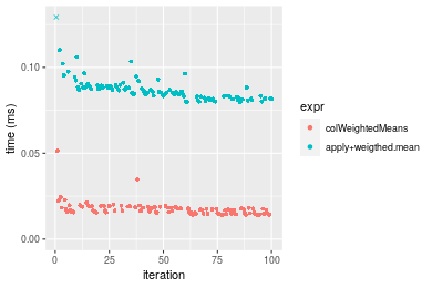
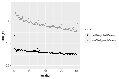
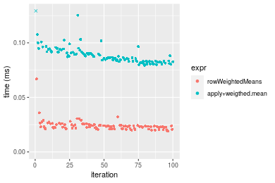Table: Benchmarking of colWeightedMeans() and rowWeightedMeans() on 10x10 data (original and transposed). The top panel shows times in milliseconds and the bottom panel shows relative times.

	expr	min	lq	mean	median	uq	max
1	colWeightedMeans	13.956	15.1095	17.39410	16.614	18.3450	51.339
2	rowWeightedMeans	19.123	21.7185	24.01519	23.250	24.8235	66.777

	expr	min	lq	mean	median	uq	max
1	colWeightedMeans	1.000000	1.000000	1.000000	1.000000	1.000000	1.000000
2	rowWeightedMeans	1.370235	1.437407	1.380651	1.399422	1.353148	1.300707

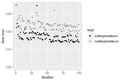
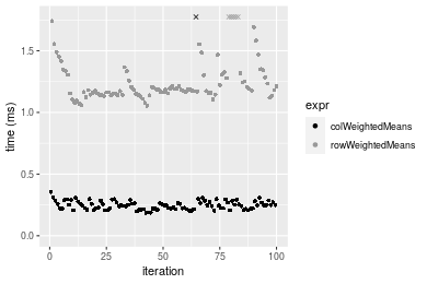
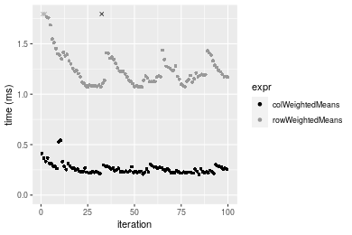
Figure: Benchmarking of colWeightedMeans() and rowWeightedMeans() on 10x10 data (original and transposed). Outliers are displayed as crosses. Times are in milliseconds.

100x100 matrix

> X <- data[["100x100"]]
> w <- runif(nrow(X))
> gc()
           used  (Mb) gc trigger  (Mb) max used  (Mb)
Ncells  5317634 284.0    8529671 455.6  8529671 455.6
Vcells 10416411  79.5   31876688 243.2 60562128 462.1
> colStats <- microbenchmark(colWeightedMeans = colWeightedMeans(X, w = w, na.rm = FALSE), `apply+weigthed.mean` = apply(X, 
+     MARGIN = 2L, FUN = weighted.mean, w = w, na.rm = FALSE), unit = "ms")
> X <- t(X)
> gc()
           used  (Mb) gc trigger  (Mb) max used  (Mb)
Ncells  5317610 284.0    8529671 455.6  8529671 455.6
Vcells 10426424  79.6   31876688 243.2 60562128 462.1
> rowStats <- microbenchmark(rowWeightedMeans = rowWeightedMeans(X, w = w, na.rm = FALSE), `apply+weigthed.mean` = apply(X, 
+     MARGIN = 1L, FUN = weighted.mean, w = w, na.rm = FALSE), unit = "ms")

Table: Benchmarking of colWeightedMeans() and apply+weigthed.mean() on 100x100 data. The top panel shows times in milliseconds and the bottom panel shows relative times.

	expr	min	lq	mean	median	uq	max
1	colWeightedMeans	0.030232	0.0341905	0.0415913	0.0396795	0.0481765	0.088324
2	apply+weigthed.mean	0.555367	0.5899205	0.7002991	0.6624400	0.7478170	1.354487

	expr	min	lq	mean	median	uq	max
1	colWeightedMeans	1.00000	1.00000	1.00000	1.00000	1.00000	1.00000
2	apply+weigthed.mean	18.37017	17.25393	16.83764	16.69477	15.52244	15.33544

Table: Benchmarking of rowWeightedMeans() and apply+weigthed.mean() on 100x100 data (transposed). The top panel shows times in milliseconds and the bottom panel shows relative times.

	expr	min	lq	mean	median	uq	max
1	rowWeightedMeans	0.119904	0.1255045	0.1474997	0.142242	0.162559	0.245560
2	apply+weigthed.mean	0.549818	0.5672270	0.6628345	0.641835	0.719392	1.138727

	expr	min	lq	mean	median	uq	max
1	rowWeightedMeans	1.000000	1.000000	1.000000	1.000000	1.000000	1.000000
2	apply+weigthed.mean	4.585485	4.519575	4.493802	4.512275	4.425421	4.637266

Figure: Benchmarking of colWeightedMeans() and apply+weigthed.mean() on 100x100 data as well as rowWeightedMeans() and apply+weigthed.mean() on the same data transposed. Outliers are displayed as crosses. Times are in milliseconds.

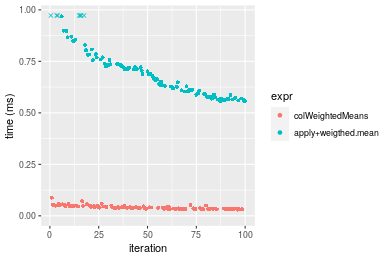
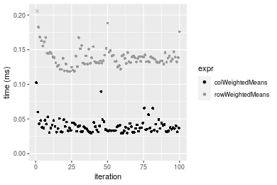
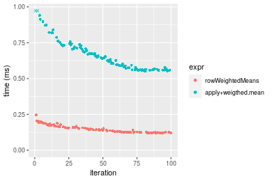Table: Benchmarking of colWeightedMeans() and rowWeightedMeans() on 100x100 data (original and transposed). The top panel shows times in milliseconds and the bottom panel shows relative times.

	expr	min	lq	mean	median	uq	max
1	colWeightedMeans	30.232	34.1905	41.59129	39.6795	48.1765	88.324
2	rowWeightedMeans	119.904	125.5045	147.49972	142.2420	162.5590	245.560

	expr	min	lq	mean	median	uq	max
1	colWeightedMeans	1.000000	1.000000	1.000000	1.000000	1.000000	1.000000
2	rowWeightedMeans	3.966129	3.670742	3.546409	3.584773	3.374239	2.780218

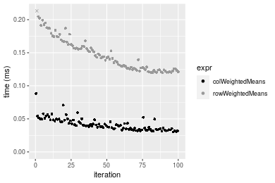
Figure: Benchmarking of colWeightedMeans() and rowWeightedMeans() on 100x100 data (original and transposed). Outliers are displayed as crosses. Times are in milliseconds.

1000x10 matrix

> X <- data[["1000x10"]]
> w <- runif(nrow(X))
> gc()
           used  (Mb) gc trigger  (Mb) max used  (Mb)
Ncells  5318335 284.1    8529671 455.6  8529671 455.6
Vcells 10420778  79.6   31876688 243.2 60562128 462.1
> colStats <- microbenchmark(colWeightedMeans = colWeightedMeans(X, w = w, na.rm = FALSE), `apply+weigthed.mean` = apply(X, 
+     MARGIN = 2L, FUN = weighted.mean, w = w, na.rm = FALSE), unit = "ms")
> X <- t(X)
> gc()
           used  (Mb) gc trigger  (Mb) max used  (Mb)
Ncells  5318329 284.1    8529671 455.6  8529671 455.6
Vcells 10430821  79.6   31876688 243.2 60562128 462.1
> rowStats <- microbenchmark(rowWeightedMeans = rowWeightedMeans(X, w = w, na.rm = FALSE), `apply+weigthed.mean` = apply(X, 
+     MARGIN = 1L, FUN = weighted.mean, w = w, na.rm = FALSE), unit = "ms")

Table: Benchmarking of colWeightedMeans() and apply+weigthed.mean() on 1000x10 data. The top panel shows times in milliseconds and the bottom panel shows relative times.

	expr	min	lq	mean	median	uq	max
1	colWeightedMeans	0.049971	0.0548630	0.0609515	0.0588590	0.0650855	0.135331
2	apply+weigthed.mean	0.211792	0.2281235	0.2468247	0.2400965	0.2623080	0.355333

	expr	min	lq	mean	median	uq	max
1	colWeightedMeans	1.000000	1.000000	1.000000	1.000000	1.000000	1.000000
2	apply+weigthed.mean	4.238298	4.158057	4.049527	4.079181	4.030206	2.625659

Table: Benchmarking of rowWeightedMeans() and apply+weigthed.mean() on 1000x10 data (transposed). The top panel shows times in milliseconds and the bottom panel shows relative times.

	expr	min	lq	mean	median	uq	max
1	rowWeightedMeans	0.152673	0.1696105	0.1855038	0.1826945	0.1975075	0.304953
2	apply+weigthed.mean	0.195234	0.2165075	0.2399114	0.2333165	0.2564390	0.351846

	expr	min	lq	mean	median	uq	max
1	rowWeightedMeans	1.000000	1.000000	1.000000	1.000000	1.000000	1.000000
2	apply+weigthed.mean	1.278772	1.276498	1.293296	1.277086	1.298376	1.153771

Figure: Benchmarking of colWeightedMeans() and apply+weigthed.mean() on 1000x10 data as well as rowWeightedMeans() and apply+weigthed.mean() on the same data transposed. Outliers are displayed as crosses. Times are in milliseconds.

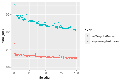
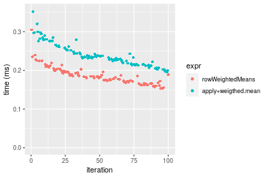Table: Benchmarking of colWeightedMeans() and rowWeightedMeans() on 1000x10 data (original and transposed). The top panel shows times in milliseconds and the bottom panel shows relative times.

	expr	min	lq	mean	median	uq	max
1	colWeightedMeans	49.971	54.8630	60.9515	58.8590	65.0855	135.331
2	rowWeightedMeans	152.673	169.6105	185.5038	182.6945	197.5075	304.953

	expr	min	lq	mean	median	uq	max
1	colWeightedMeans	1.000000	1.000000	1.000000	1.000000	1.000000	1.000000
2	rowWeightedMeans	3.055232	3.091528	3.043466	3.103935	3.034585	2.253386

Figure: Benchmarking of colWeightedMeans() and rowWeightedMeans() on 1000x10 data (original and transposed). Outliers are displayed as crosses. Times are in milliseconds.

10x1000 matrix

> X <- data[["10x1000"]]
> w <- runif(nrow(X))
> gc()
           used  (Mb) gc trigger  (Mb) max used  (Mb)
Ncells  5318551 284.1    8529671 455.6  8529671 455.6
Vcells 10420605  79.6   31876688 243.2 60562128 462.1
> colStats <- microbenchmark(colWeightedMeans = colWeightedMeans(X, w = w, na.rm = FALSE), `apply+weigthed.mean` = apply(X, 
+     MARGIN = 2L, FUN = weighted.mean, w = w, na.rm = FALSE), unit = "ms")
> X <- t(X)
> gc()
           used  (Mb) gc trigger  (Mb) max used  (Mb)
Ncells  5318527 284.1    8529671 455.6  8529671 455.6
Vcells 10430618  79.6   31876688 243.2 60562128 462.1
> rowStats <- microbenchmark(rowWeightedMeans = rowWeightedMeans(X, w = w, na.rm = FALSE), `apply+weigthed.mean` = apply(X, 
+     MARGIN = 1L, FUN = weighted.mean, w = w, na.rm = FALSE), unit = "ms")

Table: Benchmarking of colWeightedMeans() and apply+weigthed.mean() on 10x1000 data. The top panel shows times in milliseconds and the bottom panel shows relative times.

	expr	min	lq	mean	median	uq	max
1	colWeightedMeans	0.029489	0.032739	0.0394763	0.0368465	0.042318	0.10219
2	apply+weigthed.mean	4.084716	4.528123	4.8010556	4.6832870	4.777128	11.05300

	expr	min	lq	mean	median	uq	max
1	colWeightedMeans	1.0000	1.0000	1.0000	1.0000	1.0000	1.0000
2	apply+weigthed.mean	138.5166	138.3097	121.6186	127.1026	112.8864	108.1613

Table: Benchmarking of rowWeightedMeans() and apply+weigthed.mean() on 10x1000 data (transposed). The top panel shows times in milliseconds and the bottom panel shows relative times.

	expr	min	lq	mean	median	uq	max
1	rowWeightedMeans	0.118433	0.1310465	0.1392433	0.137177	0.142301	0.223296
2	apply+weigthed.mean	4.093245	4.5486995	4.8070154	4.706437	4.788188	11.003123

	expr	min	lq	mean	median	uq	max
1	rowWeightedMeans	1.00000	1.00000	1.00000	1.00000	1.00000	1.00000
2	apply+weigthed.mean	34.56169	34.71058	34.52242	34.30923	33.64831	49.27595

Figure: Benchmarking of colWeightedMeans() and apply+weigthed.mean() on 10x1000 data as well as rowWeightedMeans() and apply+weigthed.mean() on the same data transposed. Outliers are displayed as crosses. Times are in milliseconds.

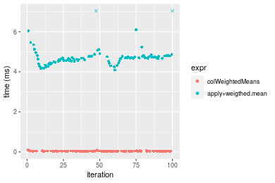
Table: Benchmarking of colWeightedMeans() and rowWeightedMeans() on 10x1000 data (original and transposed). The top panel shows times in milliseconds and the bottom panel shows relative times.

	expr	min	lq	mean	median	uq	max
1	colWeightedMeans	29.489	32.7390	39.47633	36.8465	42.318	102.190
2	rowWeightedMeans	118.433	131.0465	139.24328	137.1770	142.301	223.296

	expr	min	lq	mean	median	uq	max
1	colWeightedMeans	1.000000	1.000000	1.00000	1.000000	1.000000	1.000000
2	rowWeightedMeans	4.016176	4.002764	3.52726	3.722932	3.362659	2.185106

Figure: Benchmarking of colWeightedMeans() and rowWeightedMeans() on 10x1000 data (original and transposed). Outliers are displayed as crosses. Times are in milliseconds.

100x1000 matrix

> X <- data[["100x1000"]]
> w <- runif(nrow(X))
> gc()
           used  (Mb) gc trigger  (Mb) max used  (Mb)
Ncells  5318741 284.1    8529671 455.6  8529671 455.6
Vcells 10421196  79.6   31876688 243.2 60562128 462.1
> colStats <- microbenchmark(colWeightedMeans = colWeightedMeans(X, w = w, na.rm = FALSE), `apply+weigthed.mean` = apply(X, 
+     MARGIN = 2L, FUN = weighted.mean, w = w, na.rm = FALSE), unit = "ms")
> X <- t(X)
> gc()
           used  (Mb) gc trigger  (Mb) max used  (Mb)
Ncells  5318717 284.1    8529671 455.6  8529671 455.6
Vcells 10521209  80.3   31876688 243.2 60562128 462.1
> rowStats <- microbenchmark(rowWeightedMeans = rowWeightedMeans(X, w = w, na.rm = FALSE), `apply+weigthed.mean` = apply(X, 
+     MARGIN = 1L, FUN = weighted.mean, w = w, na.rm = FALSE), unit = "ms")

Table: Benchmarking of colWeightedMeans() and apply+weigthed.mean() on 100x1000 data. The top panel shows times in milliseconds and the bottom panel shows relative times.

	expr	min	lq	mean	median	uq	max
1	colWeightedMeans	0.185700	0.219297	0.4396765	0.2470125	0.272899	19.48006
2	apply+weigthed.mean	5.412697	5.866960	6.5537505	5.9813235	6.263001	28.49123

	expr	min	lq	mean	median	uq	max
1	colWeightedMeans	1.00000	1.00000	1.00000	1.00000	1.00000	1.000000
2	apply+weigthed.mean	29.14753	26.75349	14.90585	24.21466	22.94989	1.462584

Table: Benchmarking of rowWeightedMeans() and apply+weigthed.mean() on 100x1000 data (transposed). The top panel shows times in milliseconds and the bottom panel shows relative times.

	expr	min	lq	mean	median	uq	max
1	rowWeightedMeans	1.054020	1.153162	1.269207	1.182492	1.305193	2.109278
2	apply+weigthed.mean	5.405374	5.879766	7.117222	6.029890	6.585137	31.438123

	expr	min	lq	mean	median	uq	max
1	rowWeightedMeans	1.000000	1.000000	1.000000	1.000000	1.000000	1.00000
2	apply+weigthed.mean	5.128341	5.098821	5.607613	5.099308	5.045336	14.90468

Figure: Benchmarking of colWeightedMeans() and apply+weigthed.mean() on 100x1000 data as well as rowWeightedMeans() and apply+weigthed.mean() on the same data transposed. Outliers are displayed as crosses. Times are in milliseconds.

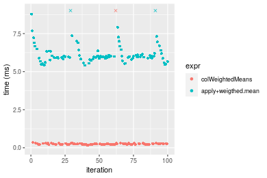
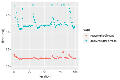Table: Benchmarking of colWeightedMeans() and rowWeightedMeans() on 100x1000 data (original and transposed). The top panel shows times in milliseconds and the bottom panel shows relative times.

	expr	min	lq	mean	median	uq	max
1	colWeightedMeans	185.70	219.297	439.6765	247.0125	272.899	19480.060
2	rowWeightedMeans	1054.02	1153.162	1269.2071	1182.4920	1305.193	2109.278

	expr	min	lq	mean	median	uq	max
1	colWeightedMeans	1.000000	1.000000	1.000000	1.000000	1.000000	1.0000000
2	rowWeightedMeans	5.675929	5.258449	2.886684	4.787175	4.782696	0.1082788

Figure: Benchmarking of colWeightedMeans() and rowWeightedMeans() on 100x1000 data (original and transposed). Outliers are displayed as crosses. Times are in milliseconds.

1000x100 matrix

> X <- data[["1000x100"]]
> w <- runif(nrow(X))
> gc()
           used  (Mb) gc trigger  (Mb) max used  (Mb)
Ncells  5318910 284.1    8529671 455.6  8529671 455.6
Vcells 10422719  79.6   31876688 243.2 60562128 462.1
> colStats <- microbenchmark(colWeightedMeans = colWeightedMeans(X, w = w, na.rm = FALSE), `apply+weigthed.mean` = apply(X, 
+     MARGIN = 2L, FUN = weighted.mean, w = w, na.rm = FALSE), unit = "ms")
> X <- t(X)
> gc()
           used  (Mb) gc trigger  (Mb) max used  (Mb)
Ncells  5318904 284.1    8529671 455.6  8529671 455.6
Vcells 10522762  80.3   31876688 243.2 60562128 462.1
> rowStats <- microbenchmark(rowWeightedMeans = rowWeightedMeans(X, w = w, na.rm = FALSE), `apply+weigthed.mean` = apply(X, 
+     MARGIN = 1L, FUN = weighted.mean, w = w, na.rm = FALSE), unit = "ms")

Table: Benchmarking of colWeightedMeans() and apply+weigthed.mean() on 1000x100 data. The top panel shows times in milliseconds and the bottom panel shows relative times.

	expr	min	lq	mean	median	uq	max
1	colWeightedMeans	0.205215	0.2276095	0.3425132	0.245658	0.2785555	8.429282
2	apply+weigthed.mean	1.540183	1.6469045	2.0503194	1.837805	2.0657935	10.520204

	expr	min	lq	mean	median	uq	max
1	colWeightedMeans	1.000000	1.000000	1.000000	1.000000	1.000000	1.000000
2	apply+weigthed.mean	7.505217	7.235658	5.986104	7.481153	7.416093	1.248055

Table: Benchmarking of rowWeightedMeans() and apply+weigthed.mean() on 1000x100 data (transposed). The top panel shows times in milliseconds and the bottom panel shows relative times.

	expr	min	lq	mean	median	uq	max
1	rowWeightedMeans	1.068420	1.125180	1.245604	1.194421	1.330394	1.94012
2	apply+weigthed.mean	1.561156	1.628209	2.060293	1.714316	1.977224	10.16854

	expr	min	lq	mean	median	uq	max
1	rowWeightedMeans	1.000000	1.000000	1.000000	1.000000	1.000000	1.000000
2	apply+weigthed.mean	1.461182	1.447065	1.654052	1.435269	1.486195	5.241191

Figure: Benchmarking of colWeightedMeans() and apply+weigthed.mean() on 1000x100 data as well as rowWeightedMeans() and apply+weigthed.mean() on the same data transposed. Outliers are displayed as crosses. Times are in milliseconds.

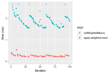
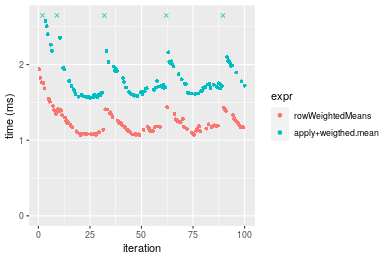Table: Benchmarking of colWeightedMeans() and rowWeightedMeans() on 1000x100 data (original and transposed). The top panel shows times in milliseconds and the bottom panel shows relative times.

	expr	min	lq	mean	median	uq	max
1	colWeightedMeans	205.215	227.6095	342.5132	245.658	278.5555	8429.282
2	rowWeightedMeans	1068.420	1125.1800	1245.6036	1194.421	1330.3935	1940.120

	expr	min	lq	mean	median	uq	max
1	colWeightedMeans	1.000000	1.000000	1.000000	1.000000	1.000000	1.0000000
2	rowWeightedMeans	5.206345	4.943467	3.636659	4.862129	4.776045	0.2301643

Figure: Benchmarking of colWeightedMeans() and rowWeightedMeans() on 1000x100 data (original and transposed). Outliers are displayed as crosses. Times are in milliseconds.

Appendix

Session information

R version 4.1.1 Patched (2021-08-10 r80727)
Platform: x86_64-pc-linux-gnu (64-bit)
Running under: Ubuntu 18.04.5 LTS

Matrix products: default
BLAS:   /home/hb/software/R-devel/R-4-1-branch/lib/R/lib/libRblas.so
LAPACK: /home/hb/software/R-devel/R-4-1-branch/lib/R/lib/libRlapack.so

locale:
 [1] LC_CTYPE=en_US.UTF-8       LC_NUMERIC=C              
 [3] LC_TIME=en_US.UTF-8        LC_COLLATE=en_US.UTF-8    
 [5] LC_MONETARY=en_US.UTF-8    LC_MESSAGES=en_US.UTF-8   
 [7] LC_PAPER=en_US.UTF-8       LC_NAME=C                 
 [9] LC_ADDRESS=C               LC_TELEPHONE=C            
[11] LC_MEASUREMENT=en_US.UTF-8 LC_IDENTIFICATION=C       

attached base packages:
[1] stats     graphics  grDevices utils     datasets  methods   base     

other attached packages:
[1] microbenchmark_1.4-7   matrixStats_0.60.1     ggplot2_3.3.5         
[4] knitr_1.33             R.devices_2.17.0       R.utils_2.10.1        
[7] R.oo_1.24.0            R.methodsS3_1.8.1-9001 history_0.0.1-9000    

loaded via a namespace (and not attached):
 [1] Biobase_2.52.0          httr_1.4.2              splines_4.1.1          
 [4] bit64_4.0.5             network_1.17.1          assertthat_0.2.1       
 [7] highr_0.9               stats4_4.1.1            blob_1.2.2             
[10] GenomeInfoDbData_1.2.6  robustbase_0.93-8       pillar_1.6.2           
[13] RSQLite_2.2.8           lattice_0.20-44         glue_1.4.2             
[16] digest_0.6.27           XVector_0.32.0          colorspace_2.0-2       
[19] Matrix_1.3-4            XML_3.99-0.7            pkgconfig_2.0.3        
[22] zlibbioc_1.38.0         genefilter_1.74.0       purrr_0.3.4            
[25] ergm_4.1.2              xtable_1.8-4            scales_1.1.1           
[28] tibble_3.1.4            annotate_1.70.0         KEGGREST_1.32.0        
[31] farver_2.1.0            generics_0.1.0          IRanges_2.26.0         
[34] ellipsis_0.3.2          cachem_1.0.6            withr_2.4.2            
[37] BiocGenerics_0.38.0     mime_0.11               survival_3.2-13        
[40] magrittr_2.0.1          crayon_1.4.1            statnet.common_4.5.0   
[43] memoise_2.0.0           laeken_0.5.1            fansi_0.5.0            
[46] R.cache_0.15.0          MASS_7.3-54             R.rsp_0.44.0           
[49] progressr_0.8.0         tools_4.1.1             lifecycle_1.0.0        
[52] S4Vectors_0.30.0        trust_0.1-8             munsell_0.5.0          
[55] tabby_0.0.1-9001        AnnotationDbi_1.54.1    Biostrings_2.60.2      
[58] compiler_4.1.1          GenomeInfoDb_1.28.1     rlang_0.4.11           
[61] grid_4.1.1              RCurl_1.98-1.4          cwhmisc_6.6            
[64] rappdirs_0.3.3          startup_0.15.0          labeling_0.4.2         
[67] bitops_1.0-7            base64enc_0.1-3         boot_1.3-28            
[70] gtable_0.3.0            DBI_1.1.1               markdown_1.1           
[73] R6_2.5.1                lpSolveAPI_5.5.2.0-17.7 rle_0.9.2              
[76] dplyr_1.0.7             fastmap_1.1.0           bit_4.0.4              
[79] utf8_1.2.2              parallel_4.1.1          Rcpp_1.0.7             
[82] vctrs_0.3.8             png_0.1-7               DEoptimR_1.0-9         
[85] tidyselect_1.1.1        xfun_0.25               coda_0.19-4            

Total processing time was 14.77 secs.

Reproducibility

To reproduce this report, do:

html <- matrixStats:::benchmark('colWeightedMeans')

---

Copyright Henrik Bengtsson. Last updated on 2021-08-25 19:11:39 (+0200 UTC). Powered by RSP.