matrixStats.benchmarks

---

colRanges() and rowRanges() benchmarks

This report benchmark the performance of colRanges() and rowRanges() against alternative methods.

Alternative methods

• apply() + range()

Data type “integer”

Data

> rmatrix <- function(nrow, ncol, mode = c("logical", "double", "integer", "index"), range = c(-100, 
+     +100), na_prob = 0) {
+     mode <- match.arg(mode)
+     n <- nrow * ncol
+     if (mode == "logical") {
+         x <- sample(c(FALSE, TRUE), size = n, replace = TRUE)
+     }     else if (mode == "index") {
+         x <- seq_len(n)
+         mode <- "integer"
+     }     else {
+         x <- runif(n, min = range[1], max = range[2])
+     }
+     storage.mode(x) <- mode
+     if (na_prob > 0) 
+         x[sample(n, size = na_prob * n)] <- NA
+     dim(x) <- c(nrow, ncol)
+     x
+ }
> rmatrices <- function(scale = 10, seed = 1, ...) {
+     set.seed(seed)
+     data <- list()
+     data[[1]] <- rmatrix(nrow = scale * 1, ncol = scale * 1, ...)
+     data[[2]] <- rmatrix(nrow = scale * 10, ncol = scale * 10, ...)
+     data[[3]] <- rmatrix(nrow = scale * 100, ncol = scale * 1, ...)
+     data[[4]] <- t(data[[3]])
+     data[[5]] <- rmatrix(nrow = scale * 10, ncol = scale * 100, ...)
+     data[[6]] <- t(data[[5]])
+     names(data) <- sapply(data, FUN = function(x) paste(dim(x), collapse = "x"))
+     data
+ }
> data <- rmatrices(mode = mode)

Results

10x10 integer matrix

> X <- data[["10x10"]]
> gc()
           used  (Mb) gc trigger  (Mb) max used  (Mb)
Ncells  5289264 282.5    8529671 455.6  8529671 455.6
Vcells 10458349  79.8   31876688 243.2 60562128 462.1
> colStats <- microbenchmark(colRanges = colRanges(X, na.rm = FALSE), `apply+range` = apply(X, MARGIN = 2L, 
+     FUN = range, na.rm = FALSE), unit = "ms")
> X <- t(X)
> gc()
           used  (Mb) gc trigger  (Mb) max used  (Mb)
Ncells  5279040 282.0    8529671 455.6  8529671 455.6
Vcells 10424711  79.6   31876688 243.2 60562128 462.1
> rowStats <- microbenchmark(rowRanges = rowRanges(X, na.rm = FALSE), `apply+range` = apply(X, MARGIN = 1L, 
+     FUN = range, na.rm = FALSE), unit = "ms")

Table: Benchmarking of colRanges() and apply+range() on integer+10x10 data. The top panel shows times in milliseconds and the bottom panel shows relative times.

	expr	min	lq	mean	median	uq	max
1	colRanges	0.002045	0.0022765	0.0030860	0.0026165	0.0035735	0.015707
2	apply+range	0.061176	0.0633180	0.0671895	0.0648315	0.0677135	0.163632

	expr	min	lq	mean	median	uq	max
1	colRanges	1.00000	1.00000	1.00000	1.00000	1.00000	1.00000
2	apply+range	29.91491	27.81375	21.77228	24.77795	18.94879	10.41778

Table: Benchmarking of rowRanges() and apply+range() on integer+10x10 data (transposed). The top panel shows times in milliseconds and the bottom panel shows relative times.

	expr	min	lq	mean	median	uq	max
1	rowRanges	0.002118	0.0024495	0.0034029	0.0033835	0.0036155	0.017028
2	apply+range	0.061230	0.0628170	0.0667048	0.0651310	0.0667565	0.156645

	expr	min	lq	mean	median	uq	max
1	rowRanges	1.00000	1.00000	1.00000	1.00000	1.00000	1.00000
2	apply+range	28.90935	25.64483	19.60211	19.24959	18.46397	9.19926

Figure: Benchmarking of colRanges() and apply+range() on integer+10x10 data as well as rowRanges() and apply+range() on the same data transposed. Outliers are displayed as crosses. Times are in milliseconds.

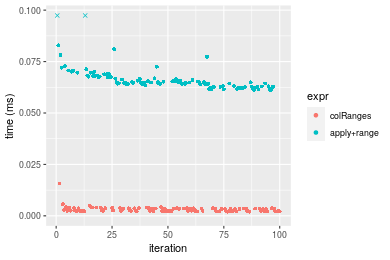
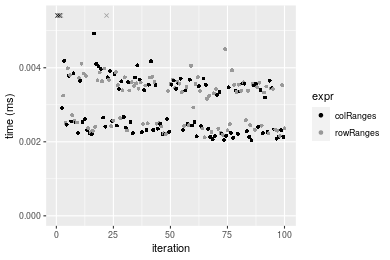
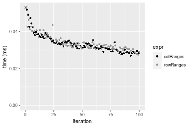
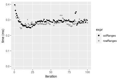
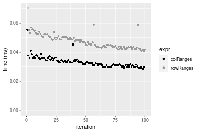
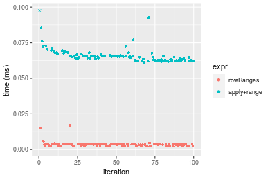Table: Benchmarking of colRanges() and rowRanges() on integer+10x10 data (original and transposed). The top panel shows times in milliseconds and the bottom panel shows relative times.

	expr	min	lq	mean	median	uq	max
1	colRanges	2.045	2.2765	3.08601	2.6165	3.5735	15.707
2	rowRanges	2.118	2.4495	3.40294	3.3835	3.6155	17.028

	expr	min	lq	mean	median	uq	max
1	colRanges	1.000000	1.000000	1.000000	1.00000	1.000000	1.000000
2	rowRanges	1.035697	1.075994	1.102699	1.29314	1.011753	1.084103

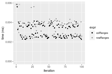
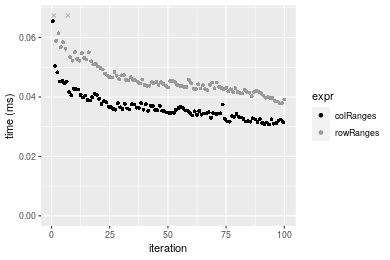
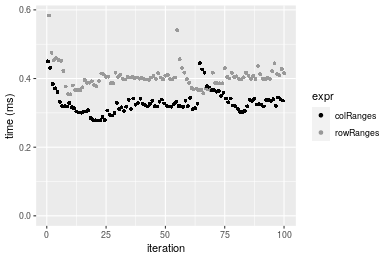
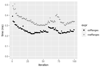
Figure: Benchmarking of colRanges() and rowRanges() on integer+10x10 data (original and transposed). Outliers are displayed as crosses. Times are in milliseconds.

100x100 integer matrix

> X <- data[["100x100"]]
> gc()
           used  (Mb) gc trigger  (Mb) max used  (Mb)
Ncells  5277618 281.9    8529671 455.6  8529671 455.6
Vcells 10041243  76.7   31876688 243.2 60562128 462.1
> colStats <- microbenchmark(colRanges = colRanges(X, na.rm = FALSE), `apply+range` = apply(X, MARGIN = 2L, 
+     FUN = range, na.rm = FALSE), unit = "ms")
> X <- t(X)
> gc()
           used  (Mb) gc trigger  (Mb) max used  (Mb)
Ncells  5277594 281.9    8529671 455.6  8529671 455.6
Vcells 10046256  76.7   31876688 243.2 60562128 462.1
> rowStats <- microbenchmark(rowRanges = rowRanges(X, na.rm = FALSE), `apply+range` = apply(X, MARGIN = 1L, 
+     FUN = range, na.rm = FALSE), unit = "ms")

Table: Benchmarking of colRanges() and apply+range() on integer+100x100 data. The top panel shows times in milliseconds and the bottom panel shows relative times.

	expr	min	lq	mean	median	uq	max
1	colRanges	0.026781	0.0303305	0.0336904	0.0322635	0.0350315	0.075468
2	apply+range	0.362779	0.3908045	0.4380096	0.4222460	0.4719190	0.713652

	expr	min	lq	mean	median	uq	max
1	colRanges	1.00000	1.00000	1.00000	1.00000	1.00000	1.000000
2	apply+range	13.54613	12.88487	13.00103	13.08742	13.47128	9.456352

Table: Benchmarking of rowRanges() and apply+range() on integer+100x100 data (transposed). The top panel shows times in milliseconds and the bottom panel shows relative times.

	expr	min	lq	mean	median	uq	max
1	rowRanges	0.027419	0.0309615	0.0338300	0.0323500	0.035481	0.054192
2	apply+range	0.357456	0.3869295	0.4280655	0.4106165	0.454320	0.675929

	expr	min	lq	mean	median	uq	max
1	rowRanges	1.0000	1.00000	1.00000	1.00000	1.0000	1.00000
2	apply+range	13.0368	12.49712	12.65341	12.69294	12.8046	12.47286

Figure: Benchmarking of colRanges() and apply+range() on integer+100x100 data as well as rowRanges() and apply+range() on the same data transposed. Outliers are displayed as crosses. Times are in milliseconds.

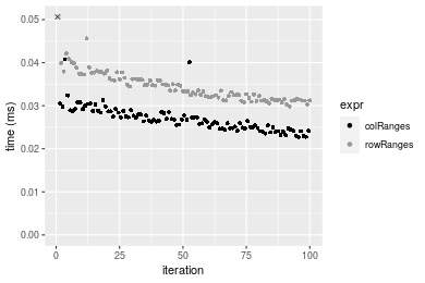
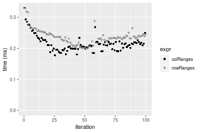
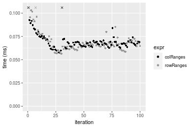
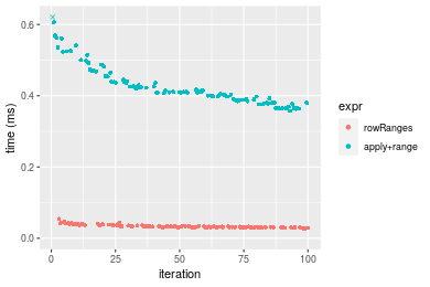Table: Benchmarking of colRanges() and rowRanges() on integer+100x100 data (original and transposed). The top panel shows times in milliseconds and the bottom panel shows relative times.

	expr	min	lq	mean	median	uq	max
1	colRanges	26.781	30.3305	33.69038	32.2635	35.0315	75.468
2	rowRanges	27.419	30.9615	33.83005	32.3500	35.4810	54.192

	expr	min	lq	mean	median	uq	max
1	colRanges	1.000000	1.000000	1.000000	1.000000	1.000000	1.0000000
2	rowRanges	1.023823	1.020804	1.004146	1.002681	1.012831	0.7180792

Figure: Benchmarking of colRanges() and rowRanges() on integer+100x100 data (original and transposed). Outliers are displayed as crosses. Times are in milliseconds.

1000x10 integer matrix

> X <- data[["1000x10"]]
> gc()
           used  (Mb) gc trigger  (Mb) max used  (Mb)
Ncells  5276992 281.9    8529671 455.6  8529671 455.6
Vcells 10019001  76.5   31876688 243.2 60562128 462.1
> colStats <- microbenchmark(colRanges = colRanges(X, na.rm = FALSE), `apply+range` = apply(X, MARGIN = 2L, 
+     FUN = range, na.rm = FALSE), unit = "ms")
> X <- t(X)
> gc()
           used  (Mb) gc trigger  (Mb) max used  (Mb)
Ncells  5276986 281.9    8529671 455.6  8529671 455.6
Vcells 10024044  76.5   31876688 243.2 60562128 462.1
> rowStats <- microbenchmark(rowRanges = rowRanges(X, na.rm = FALSE), `apply+range` = apply(X, MARGIN = 1L, 
+     FUN = range, na.rm = FALSE), unit = "ms")

Table: Benchmarking of colRanges() and apply+range() on integer+1000x10 data. The top panel shows times in milliseconds and the bottom panel shows relative times.

	expr	min	lq	mean	median	uq	max
1	colRanges	0.022732	0.0248185	0.0272224	0.0266035	0.028616	0.056743
2	apply+range	0.157993	0.1705790	0.1863602	0.1843510	0.194982	0.309690

	expr	min	lq	mean	median	uq	max
1	colRanges	1.000000	1.000000	1.000000	1.000000	1.000000	1.000000
2	apply+range	6.950246	6.873058	6.845842	6.929577	6.813741	5.457766

Table: Benchmarking of rowRanges() and apply+range() on integer+1000x10 data (transposed). The top panel shows times in milliseconds and the bottom panel shows relative times.

	expr	min	lq	mean	median	uq	max
1	rowRanges	0.02983	0.0316140	0.0344927	0.0334810	0.0361975	0.055681
2	apply+range	0.15799	0.1682565	0.1819805	0.1794215	0.1941095	0.293861

	expr	min	lq	mean	median	uq	max
1	rowRanges	1.000000	1.000000	1.00000	1.000000	1.000000	1.000000
2	apply+range	5.296346	5.322215	5.27592	5.358905	5.362511	5.277581

Figure: Benchmarking of colRanges() and apply+range() on integer+1000x10 data as well as rowRanges() and apply+range() on the same data transposed. Outliers are displayed as crosses. Times are in milliseconds.

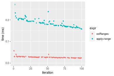
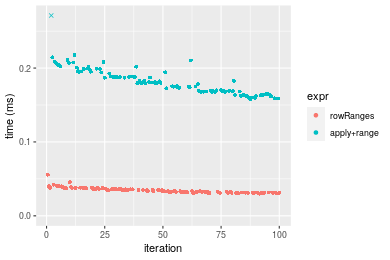Table: Benchmarking of colRanges() and rowRanges() on integer+1000x10 data (original and transposed). The top panel shows times in milliseconds and the bottom panel shows relative times.

	expr	min	lq	mean	median	uq	max
1	colRanges	22.732	24.8185	27.22240	26.6035	28.6160	56.743
2	rowRanges	29.830	31.6140	34.49266	33.4810	36.1975	55.681

	expr	min	lq	mean	median	uq	max
1	colRanges	1.000000	1.000000	1.000000	1.000000	1.000000	1.000000
2	rowRanges	1.312247	1.273808	1.267069	1.258519	1.264939	0.981284

Figure: Benchmarking of colRanges() and rowRanges() on integer+1000x10 data (original and transposed). Outliers are displayed as crosses. Times are in milliseconds.

10x1000 integer matrix

> X <- data[["10x1000"]]
> gc()
           used  (Mb) gc trigger  (Mb) max used  (Mb)
Ncells  5277198 281.9    8529671 455.6  8529671 455.6
Vcells 10019703  76.5   31876688 243.2 60562128 462.1
> colStats <- microbenchmark(colRanges = colRanges(X, na.rm = FALSE), `apply+range` = apply(X, MARGIN = 2L, 
+     FUN = range, na.rm = FALSE), unit = "ms")
> X <- t(X)
> gc()
           used  (Mb) gc trigger  (Mb) max used  (Mb)
Ncells  5277174 281.9    8529671 455.6  8529671 455.6
Vcells 10024716  76.5   31876688 243.2 60562128 462.1
> rowStats <- microbenchmark(rowRanges = rowRanges(X, na.rm = FALSE), `apply+range` = apply(X, MARGIN = 1L, 
+     FUN = range, na.rm = FALSE), unit = "ms")

Table: Benchmarking of colRanges() and apply+range() on integer+10x1000 data. The top panel shows times in milliseconds and the bottom panel shows relative times.

	expr	min	lq	mean	median	uq	max
1	colRanges	0.054437	0.061474	0.0658455	0.0641575	0.066908	0.101347
2	apply+range	2.290327	2.546572	2.7292810	2.6289990	2.779084	8.439234

	expr	min	lq	mean	median	uq	max
1	colRanges	1.00000	1.00000	1.00000	1.00000	1.00000	1.00000
2	apply+range	42.07298	41.42519	41.44977	40.97727	41.53589	83.27068

Table: Benchmarking of rowRanges() and apply+range() on integer+10x1000 data (transposed). The top panel shows times in milliseconds and the bottom panel shows relative times.

	expr	min	lq	mean	median	uq	max
1	rowRanges	0.046342	0.051257	0.054780	0.053720	0.056809	0.084516
2	apply+range	2.320344	2.543288	2.719282	2.622218	2.719834	8.373839

	expr	min	lq	mean	median	uq	max
1	rowRanges	1.00	1.00000	1.00000	1.0000	1.00000	1.00000
2	apply+range	50.07	49.61835	49.64007	48.8127	47.87681	99.07993

Figure: Benchmarking of colRanges() and apply+range() on integer+10x1000 data as well as rowRanges() and apply+range() on the same data transposed. Outliers are displayed as crosses. Times are in milliseconds.

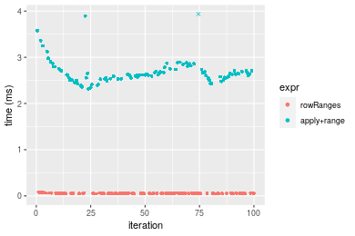Table: Benchmarking of colRanges() and rowRanges() on integer+10x1000 data (original and transposed). The top panel shows times in milliseconds and the bottom panel shows relative times.

	expr	min	lq	mean	median	uq	max
2	rowRanges	46.342	51.257	54.77998	53.7200	56.809	84.516
1	colRanges	54.437	61.474	65.84551	64.1575	66.908	101.347

	expr	min	lq	mean	median	uq	max
2	rowRanges	1.00000	1.000000	1.000	1.000000	1.000000	1.000000
1	colRanges	1.17468	1.199329	1.202	1.194295	1.177771	1.199146

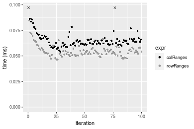
Figure: Benchmarking of colRanges() and rowRanges() on integer+10x1000 data (original and transposed). Outliers are displayed as crosses. Times are in milliseconds.

100x1000 integer matrix

> X <- data[["100x1000"]]
> gc()
           used  (Mb) gc trigger  (Mb) max used  (Mb)
Ncells  5277364 281.9    8529671 455.6  8529671 455.6
Vcells 10020150  76.5   31876688 243.2 60562128 462.1
> colStats <- microbenchmark(colRanges = colRanges(X, na.rm = FALSE), `apply+range` = apply(X, MARGIN = 2L, 
+     FUN = range, na.rm = FALSE), unit = "ms")
> X <- t(X)
> gc()
           used  (Mb) gc trigger  (Mb) max used  (Mb)
Ncells  5277358 281.9    8529671 455.6  8529671 455.6
Vcells 10070193  76.9   31876688 243.2 60562128 462.1
> rowStats <- microbenchmark(rowRanges = rowRanges(X, na.rm = FALSE), `apply+range` = apply(X, MARGIN = 1L, 
+     FUN = range, na.rm = FALSE), unit = "ms")

Table: Benchmarking of colRanges() and apply+range() on integer+100x1000 data. The top panel shows times in milliseconds and the bottom panel shows relative times.

	expr	min	lq	mean	median	uq	max
1	colRanges	0.249543	0.280823	0.2887335	0.288383	0.295516	0.397379
2	apply+range	3.116081	3.481004	3.7826471	3.574117	3.703783	21.547658

	expr	min	lq	mean	median	uq	max
1	colRanges	1.00000	1.00000	1.00000	1.00000	1.00000	1.00000
2	apply+range	12.48715	12.39572	13.10082	12.39365	12.53327	54.22445

Table: Benchmarking of rowRanges() and apply+range() on integer+100x1000 data (transposed). The top panel shows times in milliseconds and the bottom panel shows relative times.

	expr	min	lq	mean	median	uq	max
1	rowRanges	0.243785	0.2718925	0.281692	0.277003	0.287962	0.391929
2	apply+range	3.093743	3.4926325	3.814143	3.597789	3.734865	21.692554

	expr	min	lq	mean	median	uq	max
1	rowRanges	1.00000	1.00000	1.00000	1.00000	1.00000	1.00000
2	apply+range	12.69046	12.84564	13.54012	12.98827	12.96999	55.34817

Figure: Benchmarking of colRanges() and apply+range() on integer+100x1000 data as well as rowRanges() and apply+range() on the same data transposed. Outliers are displayed as crosses. Times are in milliseconds.

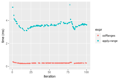
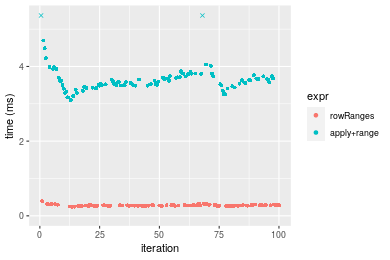Table: Benchmarking of colRanges() and rowRanges() on integer+100x1000 data (original and transposed). The top panel shows times in milliseconds and the bottom panel shows relative times.

	expr	min	lq	mean	median	uq	max
2	rowRanges	243.785	271.8925	281.6920	277.003	287.962	391.929
1	colRanges	249.543	280.8230	288.7335	288.383	295.516	397.379

	expr	min	lq	mean	median	uq	max
2	rowRanges	1.000000	1.000000	1.000000	1.000000	1.000000	1.000000
1	colRanges	1.023619	1.032846	1.024997	1.041083	1.026233	1.013906

Figure: Benchmarking of colRanges() and rowRanges() on integer+100x1000 data (original and transposed). Outliers are displayed as crosses. Times are in milliseconds.

1000x100 integer matrix

> X <- data[["1000x100"]]
> gc()
           used  (Mb) gc trigger  (Mb) max used  (Mb)
Ncells  5277556 281.9    8529671 455.6  8529671 455.6
Vcells 10020707  76.5   31876688 243.2 60562128 462.1
> colStats <- microbenchmark(colRanges = colRanges(X, na.rm = FALSE), `apply+range` = apply(X, MARGIN = 2L, 
+     FUN = range, na.rm = FALSE), unit = "ms")
> X <- t(X)
> gc()
           used  (Mb) gc trigger  (Mb) max used  (Mb)
Ncells  5277550 281.9    8529671 455.6  8529671 455.6
Vcells 10070750  76.9   31876688 243.2 60562128 462.1
> rowStats <- microbenchmark(rowRanges = rowRanges(X, na.rm = FALSE), `apply+range` = apply(X, MARGIN = 1L, 
+     FUN = range, na.rm = FALSE), unit = "ms")

Table: Benchmarking of colRanges() and apply+range() on integer+1000x100 data. The top panel shows times in milliseconds and the bottom panel shows relative times.

	expr	min	lq	mean	median	uq	max
1	colRanges	0.177355	0.198986	0.2149122	0.2100515	0.2205075	0.330149
2	apply+range	1.023167	1.124735	1.2023569	1.1665490	1.2148345	1.797137

	expr	min	lq	mean	median	uq	max
1	colRanges	1.000000	1.000000	1.000000	1.000000	1.000000	1.000000
2	apply+range	5.769034	5.652332	5.594643	5.553633	5.509266	5.443412

Table: Benchmarking of rowRanges() and apply+range() on integer+1000x100 data (transposed). The top panel shows times in milliseconds and the bottom panel shows relative times.

	expr	min	lq	mean	median	uq	max
1	rowRanges	0.200309	0.2239275	0.2363775	0.2344545	0.2448365	0.328637
2	apply+range	1.031645	1.1451460	1.2352070	1.1739475	1.2419285	2.397593

	expr	min	lq	mean	median	uq	max
1	rowRanges	1.000000	1.000000	1.000000	1.000000	1.000000	1.000000
2	apply+range	5.150268	5.113914	5.225569	5.007144	5.072481	7.295566

Figure: Benchmarking of colRanges() and apply+range() on integer+1000x100 data as well as rowRanges() and apply+range() on the same data transposed. Outliers are displayed as crosses. Times are in milliseconds.

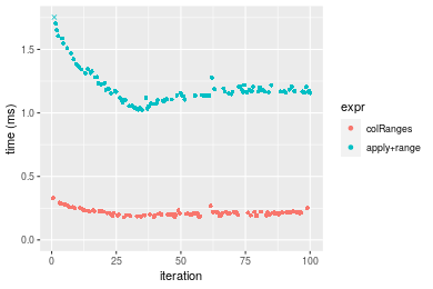
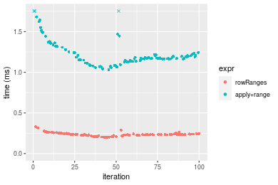Table: Benchmarking of colRanges() and rowRanges() on integer+1000x100 data (original and transposed). The top panel shows times in milliseconds and the bottom panel shows relative times.

	expr	min	lq	mean	median	uq	max
1	colRanges	177.355	198.9860	214.9122	210.0515	220.5075	330.149
2	rowRanges	200.309	223.9275	236.3775	234.4545	244.8365	328.637

	expr	min	lq	mean	median	uq	max
1	colRanges	1.000000	1.000000	1.00000	1.000000	1.000000	1.0000000
2	rowRanges	1.129424	1.125343	1.09988	1.116176	1.110332	0.9954202

Figure: Benchmarking of colRanges() and rowRanges() on integer+1000x100 data (original and transposed). Outliers are displayed as crosses. Times are in milliseconds.

Data type “double”

Data

> rmatrix <- function(nrow, ncol, mode = c("logical", "double", "integer", "index"), range = c(-100, 
+     +100), na_prob = 0) {
+     mode <- match.arg(mode)
+     n <- nrow * ncol
+     if (mode == "logical") {
+         x <- sample(c(FALSE, TRUE), size = n, replace = TRUE)
+     }     else if (mode == "index") {
+         x <- seq_len(n)
+         mode <- "integer"
+     }     else {
+         x <- runif(n, min = range[1], max = range[2])
+     }
+     storage.mode(x) <- mode
+     if (na_prob > 0) 
+         x[sample(n, size = na_prob * n)] <- NA
+     dim(x) <- c(nrow, ncol)
+     x
+ }
> rmatrices <- function(scale = 10, seed = 1, ...) {
+     set.seed(seed)
+     data <- list()
+     data[[1]] <- rmatrix(nrow = scale * 1, ncol = scale * 1, ...)
+     data[[2]] <- rmatrix(nrow = scale * 10, ncol = scale * 10, ...)
+     data[[3]] <- rmatrix(nrow = scale * 100, ncol = scale * 1, ...)
+     data[[4]] <- t(data[[3]])
+     data[[5]] <- rmatrix(nrow = scale * 10, ncol = scale * 100, ...)
+     data[[6]] <- t(data[[5]])
+     names(data) <- sapply(data, FUN = function(x) paste(dim(x), collapse = "x"))
+     data
+ }
> data <- rmatrices(mode = mode)

Results

10x10 double matrix

> X <- data[["10x10"]]
> gc()
           used  (Mb) gc trigger  (Mb) max used  (Mb)
Ncells  5277774 281.9    8529671 455.6  8529671 455.6
Vcells 10137112  77.4   31876688 243.2 60562128 462.1
> colStats <- microbenchmark(colRanges = colRanges(X, na.rm = FALSE), `apply+range` = apply(X, MARGIN = 2L, 
+     FUN = range, na.rm = FALSE), unit = "ms")
> X <- t(X)
> gc()
           used  (Mb) gc trigger  (Mb) max used  (Mb)
Ncells  5277741 281.9    8529671 455.6  8529671 455.6
Vcells 10137210  77.4   31876688 243.2 60562128 462.1
> rowStats <- microbenchmark(rowRanges = rowRanges(X, na.rm = FALSE), `apply+range` = apply(X, MARGIN = 1L, 
+     FUN = range, na.rm = FALSE), unit = "ms")

Table: Benchmarking of colRanges() and apply+range() on double+10x10 data. The top panel shows times in milliseconds and the bottom panel shows relative times.

	expr	min	lq	mean	median	uq	max
1	colRanges	0.002259	0.0025155	0.0032496	0.0029085	0.0036680	0.015910
2	apply+range	0.062972	0.0655225	0.0685291	0.0670195	0.0684135	0.156534

	expr	min	lq	mean	median	uq	max
1	colRanges	1.00000	1.00000	1.00000	1.00000	1.00000	1.000000
2	apply+range	27.87605	26.04751	21.08828	23.04263	18.65144	9.838718

Table: Benchmarking of rowRanges() and apply+range() on double+10x10 data (transposed). The top panel shows times in milliseconds and the bottom panel shows relative times.

	expr	min	lq	mean	median	uq	max
1	rowRanges	0.002354	0.002694	0.0036362	0.0038170	0.0039900	0.015200
2	apply+range	0.062247	0.064034	0.0678588	0.0660175	0.0672285	0.175182

	expr	min	lq	mean	median	uq	max
1	rowRanges	1.00000	1.00000	1.000	1.00000	1.00000	1.00000
2	apply+range	26.44308	23.76912	18.662	17.29565	16.84925	11.52513

Figure: Benchmarking of colRanges() and apply+range() on double+10x10 data as well as rowRanges() and apply+range() on the same data transposed. Outliers are displayed as crosses. Times are in milliseconds.

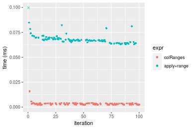
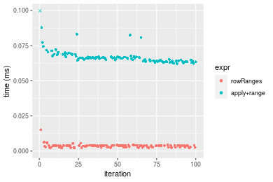Table: Benchmarking of colRanges() and rowRanges() on double+10x10 data (original and transposed). The top panel shows times in milliseconds and the bottom panel shows relative times.

	expr	min	lq	mean	median	uq	max
1	colRanges	2.259	2.5155	3.24963	2.9085	3.668	15.91
2	rowRanges	2.354	2.6940	3.63620	3.8170	3.990	15.20

	expr	min	lq	mean	median	uq	max
1	colRanges	1.000000	1.00000	1.000000	1.00000	1.000000	1.000000
2	rowRanges	1.042054	1.07096	1.118958	1.31236	1.087786	0.955374

Figure: Benchmarking of colRanges() and rowRanges() on double+10x10 data (original and transposed). Outliers are displayed as crosses. Times are in milliseconds.

100x100 double matrix

> X <- data[["100x100"]]
> gc()
           used  (Mb) gc trigger  (Mb) max used  (Mb)
Ncells  5277954 281.9    8529671 455.6  8529671 455.6
Vcells 10137224  77.4   31876688 243.2 60562128 462.1
> colStats <- microbenchmark(colRanges = colRanges(X, na.rm = FALSE), `apply+range` = apply(X, MARGIN = 2L, 
+     FUN = range, na.rm = FALSE), unit = "ms")
> X <- t(X)
> gc()
           used  (Mb) gc trigger  (Mb) max used  (Mb)
Ncells  5277930 281.9    8529671 455.6  8529671 455.6
Vcells 10147237  77.5   31876688 243.2 60562128 462.1
> rowStats <- microbenchmark(rowRanges = rowRanges(X, na.rm = FALSE), `apply+range` = apply(X, MARGIN = 1L, 
+     FUN = range, na.rm = FALSE), unit = "ms")

Table: Benchmarking of colRanges() and apply+range() on double+100x100 data. The top panel shows times in milliseconds and the bottom panel shows relative times.

	expr	min	lq	mean	median	uq	max
1	colRanges	0.030750	0.0334665	0.0365070	0.0355485	0.0377880	0.065516
2	apply+range	0.363406	0.3928520	0.4364423	0.4180270	0.4584745	0.668450

	expr	min	lq	mean	median	uq	max
1	colRanges	1.00000	1.00000	1.00000	1.00000	1.00000	1.00000
2	apply+range	11.81808	11.73866	11.95502	11.75934	12.13281	10.20285

Table: Benchmarking of rowRanges() and apply+range() on double+100x100 data (transposed). The top panel shows times in milliseconds and the bottom panel shows relative times.

	expr	min	lq	mean	median	uq	max
1	rowRanges	0.037889	0.0425985	0.0460512	0.044444	0.0472870	0.070815
2	apply+range	0.357126	0.3903375	0.4330396	0.419954	0.4560095	0.704440

	expr	min	lq	mean	median	uq	max
1	rowRanges	1.000000	1.000000	1.000000	1.00000	1.000000	1.00000
2	apply+range	9.425585	9.163175	9.403437	9.44906	9.643443	9.94761

Figure: Benchmarking of colRanges() and apply+range() on double+100x100 data as well as rowRanges() and apply+range() on the same data transposed. Outliers are displayed as crosses. Times are in milliseconds.

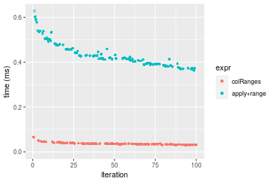
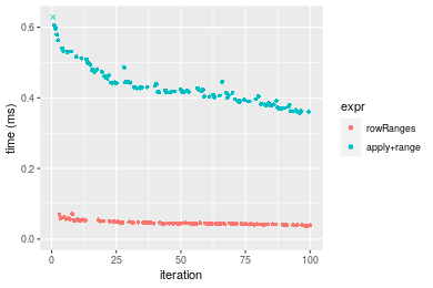Table: Benchmarking of colRanges() and rowRanges() on double+100x100 data (original and transposed). The top panel shows times in milliseconds and the bottom panel shows relative times.

	expr	min	lq	mean	median	uq	max
1	colRanges	30.750	33.4665	36.50703	35.5485	37.788	65.516
2	rowRanges	37.889	42.5985	46.05121	44.4440	47.287	70.815

	expr	min	lq	mean	median	uq	max
1	colRanges	1.000000	1.00000	1.000000	1.000000	1.000000	1.000000
2	rowRanges	1.232163	1.27287	1.261434	1.250236	1.251376	1.080881

Figure: Benchmarking of colRanges() and rowRanges() on double+100x100 data (original and transposed). Outliers are displayed as crosses. Times are in milliseconds.

1000x10 double matrix

> X <- data[["1000x10"]]
> gc()
           used  (Mb) gc trigger  (Mb) max used  (Mb)
Ncells  5278144 281.9    8529671 455.6  8529671 455.6
Vcells 10138108  77.4   31876688 243.2 60562128 462.1
> colStats <- microbenchmark(colRanges = colRanges(X, na.rm = FALSE), `apply+range` = apply(X, MARGIN = 2L, 
+     FUN = range, na.rm = FALSE), unit = "ms")
> X <- t(X)
> gc()
           used  (Mb) gc trigger  (Mb) max used  (Mb)
Ncells  5278120 281.9    8529671 455.6  8529671 455.6
Vcells 10148121  77.5   31876688 243.2 60562128 462.1
> rowStats <- microbenchmark(rowRanges = rowRanges(X, na.rm = FALSE), `apply+range` = apply(X, MARGIN = 1L, 
+     FUN = range, na.rm = FALSE), unit = "ms")

Table: Benchmarking of colRanges() and apply+range() on double+1000x10 data. The top panel shows times in milliseconds and the bottom panel shows relative times.

	expr	min	lq	mean	median	uq	max
1	colRanges	0.028562	0.0308550	0.0331219	0.032685	0.0344220	0.055471
2	apply+range	0.167954	0.1767545	0.1925280	0.189582	0.2037205	0.319261

	expr	min	lq	mean	median	uq	max
1	colRanges	1.000000	1.000000	1.000000	1.000000	1.000000	1.000000
2	apply+range	5.880331	5.728553	5.812704	5.800275	5.918323	5.755458

Table: Benchmarking of rowRanges() and apply+range() on double+1000x10 data (transposed). The top panel shows times in milliseconds and the bottom panel shows relative times.

	expr	min	lq	mean	median	uq	max
1	rowRanges	0.040850	0.043525	0.0475016	0.0467705	0.050153	0.071758
2	apply+range	0.168492	0.176742	0.1954258	0.1936765	0.207414	0.313195

	expr	min	lq	mean	median	uq	max
1	rowRanges	1.000000	1.000000	1.000000	1.000000	1.000000	1.0000
2	apply+range	4.124651	4.060701	4.114085	4.140997	4.135625	4.3646

Figure: Benchmarking of colRanges() and apply+range() on double+1000x10 data as well as rowRanges() and apply+range() on the same data transposed. Outliers are displayed as crosses. Times are in milliseconds.

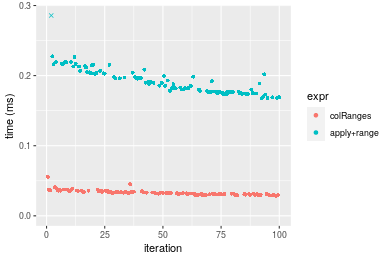
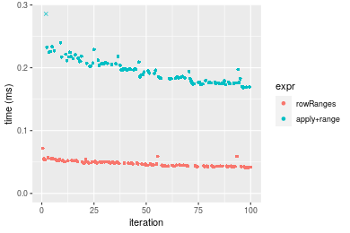Table: Benchmarking of colRanges() and rowRanges() on double+1000x10 data (original and transposed). The top panel shows times in milliseconds and the bottom panel shows relative times.

	expr	min	lq	mean	median	uq	max
1	colRanges	28.562	30.855	33.12193	32.6850	34.422	55.471
2	rowRanges	40.850	43.525	47.50163	46.7705	50.153	71.758

	expr	min	lq	mean	median	uq	max
1	colRanges	1.000000	1.00000	1.000000	1.000000	1.000000	1.000000
2	rowRanges	1.430222	1.41063	1.434144	1.430947	1.457004	1.293613

Figure: Benchmarking of colRanges() and rowRanges() on double+1000x10 data (original and transposed). Outliers are displayed as crosses. Times are in milliseconds.

10x1000 double matrix

> X <- data[["10x1000"]]
> gc()
           used  (Mb) gc trigger  (Mb) max used  (Mb)
Ncells  5278332 281.9    8529671 455.6  8529671 455.6
Vcells 10139134  77.4   31876688 243.2 60562128 462.1
> colStats <- microbenchmark(colRanges = colRanges(X, na.rm = FALSE), `apply+range` = apply(X, MARGIN = 2L, 
+     FUN = range, na.rm = FALSE), unit = "ms")
> X <- t(X)
> gc()
           used  (Mb) gc trigger  (Mb) max used  (Mb)
Ncells  5278308 281.9    8529671 455.6  8529671 455.6
Vcells 10149147  77.5   31876688 243.2 60562128 462.1
> rowStats <- microbenchmark(rowRanges = rowRanges(X, na.rm = FALSE), `apply+range` = apply(X, MARGIN = 1L, 
+     FUN = range, na.rm = FALSE), unit = "ms")

Table: Benchmarking of colRanges() and apply+range() on double+10x1000 data. The top panel shows times in milliseconds and the bottom panel shows relative times.

	expr	min	lq	mean	median	uq	max
1	colRanges	0.057283	0.064676	0.069646	0.0675615	0.070842	0.119783
2	apply+range	2.247675	2.468546	2.660573	2.5749150	2.682983	8.522724

	expr	min	lq	mean	median	uq	max
1	colRanges	1.00000	1.00000	1.00000	1.00000	1.00000	1.00000
2	apply+range	39.23808	38.16788	38.20137	38.11216	37.87277	71.15137

Table: Benchmarking of rowRanges() and apply+range() on double+10x1000 data (transposed). The top panel shows times in milliseconds and the bottom panel shows relative times.

	expr	min	lq	mean	median	uq	max
1	rowRanges	0.056377	0.063584	0.0692046	0.0663985	0.070420	0.115403
2	apply+range	2.216160	2.449838	2.6963183	2.5616395	2.741758	8.571219

	expr	min	lq	mean	median	uq	max
1	rowRanges	1.00000	1.00000	1.00000	1.00000	1.00000	1.00000
2	apply+range	39.30965	38.52915	38.96153	38.57978	38.93437	74.27206

Figure: Benchmarking of colRanges() and apply+range() on double+10x1000 data as well as rowRanges() and apply+range() on the same data transposed. Outliers are displayed as crosses. Times are in milliseconds.

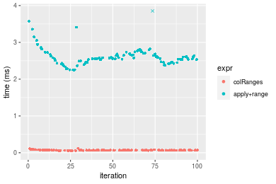
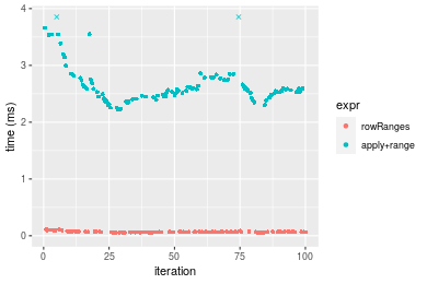Table: Benchmarking of colRanges() and rowRanges() on double+10x1000 data (original and transposed). The top panel shows times in milliseconds and the bottom panel shows relative times.

	expr	min	lq	mean	median	uq	max
2	rowRanges	56.377	63.584	69.20463	66.3985	70.420	115.403
1	colRanges	57.283	64.676	69.64601	67.5615	70.842	119.783

	expr	min	lq	mean	median	uq	max
2	rowRanges	1.00000	1.000000	1.000000	1.000000	1.000000	1.000000
1	colRanges	1.01607	1.017174	1.006378	1.017516	1.005993	1.037954

Figure: Benchmarking of colRanges() and rowRanges() on double+10x1000 data (original and transposed). Outliers are displayed as crosses. Times are in milliseconds.

100x1000 double matrix

> X <- data[["100x1000"]]
> gc()
           used  (Mb) gc trigger  (Mb) max used  (Mb)
Ncells  5278498 282.0    8529671 455.6  8529671 455.6
Vcells 10139225  77.4   31876688 243.2 60562128 462.1
> colStats <- microbenchmark(colRanges = colRanges(X, na.rm = FALSE), `apply+range` = apply(X, MARGIN = 2L, 
+     FUN = range, na.rm = FALSE), unit = "ms")
> X <- t(X)
> gc()
           used  (Mb) gc trigger  (Mb) max used  (Mb)
Ncells  5278492 282.0    8529671 455.6  8529671 455.6
Vcells 10239268  78.2   31876688 243.2 60562128 462.1
> rowStats <- microbenchmark(rowRanges = rowRanges(X, na.rm = FALSE), `apply+range` = apply(X, MARGIN = 1L, 
+     FUN = range, na.rm = FALSE), unit = "ms")

Table: Benchmarking of colRanges() and apply+range() on double+100x1000 data. The top panel shows times in milliseconds and the bottom panel shows relative times.

	expr	min	lq	mean	median	uq	max
1	colRanges	0.277662	0.312648	0.329746	0.3238985	0.338983	0.449944
2	apply+range	3.073474	3.489064	3.793124	3.5592790	3.618731	23.295720

	expr	min	lq	mean	median	uq	max
1	colRanges	1.00000	1.00000	1.00000	1.00000	1.00000	1.00000
2	apply+range	11.06912	11.15972	11.50317	10.98887	10.67526	51.77471

Table: Benchmarking of rowRanges() and apply+range() on double+100x1000 data (transposed). The top panel shows times in milliseconds and the bottom panel shows relative times.

	expr	min	lq	mean	median	uq	max
1	rowRanges	0.353825	0.3876175	0.4041883	0.400344	0.412531	0.583608
2	apply+range	3.140982	3.4950920	3.8241917	3.560674	3.664349	23.747830

	expr	min	lq	mean	median	uq	max
1	rowRanges	1.000000	1.000000	1.000000	1.000000	1.000000	1.00000
2	apply+range	8.877219	9.016858	9.461411	8.894035	8.882603	40.69141

Figure: Benchmarking of colRanges() and apply+range() on double+100x1000 data as well as rowRanges() and apply+range() on the same data transposed. Outliers are displayed as crosses. Times are in milliseconds.

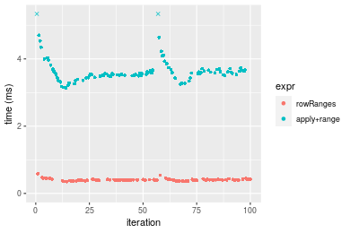Table: Benchmarking of colRanges() and rowRanges() on double+100x1000 data (original and transposed). The top panel shows times in milliseconds and the bottom panel shows relative times.

	expr	min	lq	mean	median	uq	max
1	colRanges	277.662	312.6480	329.7460	323.8985	338.983	449.944
2	rowRanges	353.825	387.6175	404.1883	400.3440	412.531	583.608

	expr	min	lq	mean	median	uq	max
1	colRanges	1.000000	1.000000	1.000000	1.000000	1.000000	1.000000
2	rowRanges	1.274301	1.239789	1.225756	1.236017	1.216967	1.297068

Figure: Benchmarking of colRanges() and rowRanges() on double+100x1000 data (original and transposed). Outliers are displayed as crosses. Times are in milliseconds.

1000x100 double matrix

> X <- data[["1000x100"]]
> gc()
           used  (Mb) gc trigger  (Mb) max used  (Mb)
Ncells  5278696 282.0    8529671 455.6  8529671 455.6
Vcells 10140447  77.4   31876688 243.2 60562128 462.1
> colStats <- microbenchmark(colRanges = colRanges(X, na.rm = FALSE), `apply+range` = apply(X, MARGIN = 2L, 
+     FUN = range, na.rm = FALSE), unit = "ms")
> X <- t(X)
> gc()
           used  (Mb) gc trigger  (Mb) max used  (Mb)
Ncells  5278684 282.0    8529671 455.6  8529671 455.6
Vcells 10240480  78.2   31876688 243.2 60562128 462.1
> rowStats <- microbenchmark(rowRanges = rowRanges(X, na.rm = FALSE), `apply+range` = apply(X, MARGIN = 1L, 
+     FUN = range, na.rm = FALSE), unit = "ms")

Table: Benchmarking of colRanges() and apply+range() on double+1000x100 data. The top panel shows times in milliseconds and the bottom panel shows relative times.

	expr	min	lq	mean	median	uq	max
1	colRanges	0.218963	0.2317655	0.2530273	0.242969	0.2717755	0.390991
2	apply+range	1.110040	1.1862190	1.3785878	1.243577	1.3958095	8.763839

	expr	min	lq	mean	median	uq	max
1	colRanges	1.000000	1.000000	1.000000	1.000000	1.000000	1.00000
2	apply+range	5.069532	5.118186	5.448377	5.118252	5.135892	22.41443

Table: Benchmarking of rowRanges() and apply+range() on double+1000x100 data (transposed). The top panel shows times in milliseconds and the bottom panel shows relative times.

	expr	min	lq	mean	median	uq	max
1	rowRanges	0.301763	0.316280	0.3493902	0.337249	0.3681175	0.672985
2	apply+range	1.152037	1.230333	1.4392455	1.277540	1.4329070	8.812583

	expr	min	lq	mean	median	uq	max
1	rowRanges	1.000000	1.000000	1.000000	1.00000	1.000000	1.00000
2	apply+range	3.817688	3.890014	4.119307	3.78812	3.892526	13.09477

Figure: Benchmarking of colRanges() and apply+range() on double+1000x100 data as well as rowRanges() and apply+range() on the same data transposed. Outliers are displayed as crosses. Times are in milliseconds.

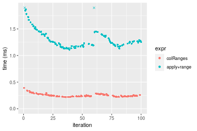
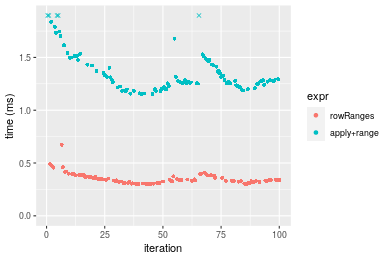Table: Benchmarking of colRanges() and rowRanges() on double+1000x100 data (original and transposed). The top panel shows times in milliseconds and the bottom panel shows relative times.

	expr	min	lq	mean	median	uq	max
1	colRanges	218.963	231.7655	253.0273	242.969	271.7755	390.991
2	rowRanges	301.763	316.2800	349.3902	337.249	368.1175	672.985

	expr	min	lq	mean	median	uq	max
1	colRanges	1.000000	1.000000	1.00000	1.000000	1.000000	1.000000
2	rowRanges	1.378146	1.364655	1.38084	1.388033	1.354491	1.721229

Figure: Benchmarking of colRanges() and rowRanges() on double+1000x100 data (original and transposed). Outliers are displayed as crosses. Times are in milliseconds.

Appendix

Session information

R version 4.1.1 Patched (2021-08-10 r80727)
Platform: x86_64-pc-linux-gnu (64-bit)
Running under: Ubuntu 18.04.5 LTS

Matrix products: default
BLAS:   /home/hb/software/R-devel/R-4-1-branch/lib/R/lib/libRblas.so
LAPACK: /home/hb/software/R-devel/R-4-1-branch/lib/R/lib/libRlapack.so

locale:
 [1] LC_CTYPE=en_US.UTF-8       LC_NUMERIC=C              
 [3] LC_TIME=en_US.UTF-8        LC_COLLATE=en_US.UTF-8    
 [5] LC_MONETARY=en_US.UTF-8    LC_MESSAGES=en_US.UTF-8   
 [7] LC_PAPER=en_US.UTF-8       LC_NAME=C                 
 [9] LC_ADDRESS=C               LC_TELEPHONE=C            
[11] LC_MEASUREMENT=en_US.UTF-8 LC_IDENTIFICATION=C       

attached base packages:
[1] stats     graphics  grDevices utils     datasets  methods   base     

other attached packages:
[1] microbenchmark_1.4-7   matrixStats_0.60.1     ggplot2_3.3.5         
[4] knitr_1.33             R.devices_2.17.0       R.utils_2.10.1        
[7] R.oo_1.24.0            R.methodsS3_1.8.1-9001 history_0.0.1-9000    

loaded via a namespace (and not attached):
 [1] Biobase_2.52.0          httr_1.4.2              splines_4.1.1          
 [4] bit64_4.0.5             network_1.17.1          assertthat_0.2.1       
 [7] highr_0.9               stats4_4.1.1            blob_1.2.2             
[10] GenomeInfoDbData_1.2.6  robustbase_0.93-8       pillar_1.6.2           
[13] RSQLite_2.2.8           lattice_0.20-44         glue_1.4.2             
[16] digest_0.6.27           XVector_0.32.0          colorspace_2.0-2       
[19] Matrix_1.3-4            XML_3.99-0.7            pkgconfig_2.0.3        
[22] zlibbioc_1.38.0         genefilter_1.74.0       purrr_0.3.4            
[25] ergm_4.1.2              xtable_1.8-4            scales_1.1.1           
[28] tibble_3.1.4            annotate_1.70.0         KEGGREST_1.32.0        
[31] farver_2.1.0            generics_0.1.0          IRanges_2.26.0         
[34] ellipsis_0.3.2          cachem_1.0.6            withr_2.4.2            
[37] BiocGenerics_0.38.0     mime_0.11               survival_3.2-13        
[40] magrittr_2.0.1          crayon_1.4.1            statnet.common_4.5.0   
[43] memoise_2.0.0           laeken_0.5.1            fansi_0.5.0            
[46] R.cache_0.15.0          MASS_7.3-54             R.rsp_0.44.0           
[49] progressr_0.8.0         tools_4.1.1             lifecycle_1.0.0        
[52] S4Vectors_0.30.0        trust_0.1-8             munsell_0.5.0          
[55] tabby_0.0.1-9001        AnnotationDbi_1.54.1    Biostrings_2.60.2      
[58] compiler_4.1.1          GenomeInfoDb_1.28.1     rlang_0.4.11           
[61] grid_4.1.1              RCurl_1.98-1.4          cwhmisc_6.6            
[64] rappdirs_0.3.3          startup_0.15.0          labeling_0.4.2         
[67] bitops_1.0-7            base64enc_0.1-3         boot_1.3-28            
[70] gtable_0.3.0            DBI_1.1.1               markdown_1.1           
[73] R6_2.5.1                lpSolveAPI_5.5.2.0-17.7 rle_0.9.2              
[76] dplyr_1.0.7             fastmap_1.1.0           bit_4.0.4              
[79] utf8_1.2.2              parallel_4.1.1          Rcpp_1.0.7             
[82] vctrs_0.3.8             png_0.1-7               DEoptimR_1.0-9         
[85] tidyselect_1.1.1        xfun_0.25               coda_0.19-4            

Total processing time was 26.2 secs.

Reproducibility

To reproduce this report, do:

html <- matrixStats:::benchmark('colRanges')

---

Copyright Henrik Bengtsson. Last updated on 2021-08-25 19:07:24 (+0200 UTC). Powered by RSP.