matrixStats.benchmarks

colQuantiles() and rowQuantiles() benchmarks on subsetted computation

This report benchmark the performance of colQuantiles() and rowQuantiles() on subsetted computation.

Data

> rmatrix <- function(nrow, ncol, mode = c("logical", "double", "integer", "index"), range = c(-100, 
+     +100), na_prob = 0) {
+     mode <- match.arg(mode)
+     n <- nrow * ncol
+     if (mode == "logical") {
+         x <- sample(c(FALSE, TRUE), size = n, replace = TRUE)
+     }     else if (mode == "index") {
+         x <- seq_len(n)
+         mode <- "integer"
+     }     else {
+         x <- runif(n, min = range[1], max = range[2])
+     }
+     storage.mode(x) <- mode
+     if (na_prob > 0) 
+         x[sample(n, size = na_prob * n)] <- NA
+     dim(x) <- c(nrow, ncol)
+     x
+ }
> rmatrices <- function(scale = 10, seed = 1, ...) {
+     set.seed(seed)
+     data <- list()
+     data[[1]] <- rmatrix(nrow = scale * 1, ncol = scale * 1, ...)
+     data[[2]] <- rmatrix(nrow = scale * 10, ncol = scale * 10, ...)
+     data[[3]] <- rmatrix(nrow = scale * 100, ncol = scale * 1, ...)
+     data[[4]] <- t(data[[3]])
+     data[[5]] <- rmatrix(nrow = scale * 10, ncol = scale * 100, ...)
+     data[[6]] <- t(data[[5]])
+     names(data) <- sapply(data, FUN = function(x) paste(dim(x), collapse = "x"))
+     data
+ }
> data <- rmatrices(mode = "double")

Results

10x10 matrix

> X <- data[["10x10"]]
> rows <- sample.int(nrow(X), size = nrow(X) * 0.7)
> cols <- sample.int(ncol(X), size = ncol(X) * 0.7)
> X_S <- X[rows, cols]
> gc()
           used  (Mb) gc trigger  (Mb) max used  (Mb)
Ncells  5277191 281.9    8529671 455.6  8529671 455.6
Vcells 10438339  79.7   31876688 243.2 60562128 462.1
> probs <- seq(from = 0, to = 1, by = 0.25)
> colStats <- microbenchmark(colQuantiles_X_S = colQuantiles(X_S, probs = probs, na.rm = FALSE), `colQuantiles(X, rows, cols)` = colQuantiles(X, 
+     rows = rows, cols = cols, probs = probs, na.rm = FALSE), `colQuantiles(X[rows, cols])` = colQuantiles(X[rows, 
+     cols], probs = probs, na.rm = FALSE), unit = "ms")
> X <- t(X)
> X_S <- t(X_S)
> gc()
           used  (Mb) gc trigger  (Mb) max used  (Mb)
Ncells  5269002 281.4    8529671 455.6  8529671 455.6
Vcells 10410708  79.5   31876688 243.2 60562128 462.1
> rowStats <- microbenchmark(rowQuantiles_X_S = rowQuantiles(X_S, probs = probs, na.rm = FALSE), `rowQuantiles(X, cols, rows)` = rowQuantiles(X, 
+     rows = cols, cols = rows, probs = probs, na.rm = FALSE), `rowQuantiles(X[cols, rows])` = rowQuantiles(X[cols, 
+     rows], probs = probs, na.rm = FALSE), unit = "ms")

Table: Benchmarking of colQuantiles_X_S(), colQuantiles(X, rows, cols)() and colQuantiles(X[rows, cols])() on 10x10 data. The top panel shows times in milliseconds and the bottom panel shows relative times.

	expr	min	lq	mean	median	uq	max
3	colQuantiles(X[rows, cols])	0.189556	0.2023435	0.2312232	0.2225175	0.2461560	0.325888
2	colQuantiles(X, rows, cols)	0.190022	0.2017890	0.2369091	0.2291760	0.2614565	0.320707
1	colQuantiles_X_S	0.188130	0.2022575	0.2423824	0.2351850	0.2569375	0.975538

	expr	min	lq	mean	median	uq	max
3	colQuantiles(X[rows, cols])	1.0000000	1.0000000	1.000000	1.000000	1.000000	1.0000000
2	colQuantiles(X, rows, cols)	1.0024584	0.9972596	1.024590	1.029923	1.062158	0.9841019
1	colQuantiles_X_S	0.9924772	0.9995750	1.048261	1.056928	1.043799	2.9934763

Table: Benchmarking of rowQuantiles_X_S(), rowQuantiles(X, cols, rows)() and rowQuantiles(X[cols, rows])() on 10x10 data (transposed). The top panel shows times in milliseconds and the bottom panel shows relative times.

	expr	min	lq	mean	median	uq	max
3	rowQuantiles(X[cols, rows])	0.190946	0.2031980	0.2336701	0.2281225	0.2493630	0.332234
1	rowQuantiles_X_S	0.187947	0.2053835	0.2429414	0.2378675	0.2673165	0.334525
2	rowQuantiles(X, cols, rows)	0.190509	0.2066295	0.2489178	0.2407855	0.2598540	1.031073

	expr	min	lq	mean	median	uq	max
3	rowQuantiles(X[cols, rows])	1.0000000	1.000000	1.000000	1.000000	1.000000	1.000000
1	rowQuantiles_X_S	0.9842940	1.010755	1.039677	1.042718	1.071997	1.006896
2	rowQuantiles(X, cols, rows)	0.9977114	1.016887	1.065253	1.055510	1.042071	3.103454

Figure: Benchmarking of colQuantiles_X_S(), colQuantiles(X, rows, cols)() and colQuantiles(X[rows, cols])() on 10x10 data as well as rowQuantiles_X_S(), rowQuantiles(X, cols, rows)() and rowQuantiles(X[cols, rows])() on the same data transposed. Outliers are displayed as crosses. Times are in milliseconds.

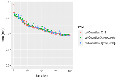
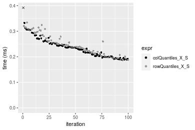
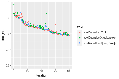Table: Benchmarking of colQuantiles_X_S() and rowQuantiles_X_S() on 10x10 data (original and transposed). The top panel shows times in milliseconds and the bottom panel shows relative times.

	expr	min	lq	mean	median	uq	max
1	colQuantiles_X_S	188.130	202.2575	242.3824	235.1850	256.9375	975.538
2	rowQuantiles_X_S	187.947	205.3835	242.9414	237.8675	267.3165	334.525

	expr	min	lq	mean	median	uq	max
1	colQuantiles_X_S	1.0000000	1.000000	1.000000	1.000000	1.000000	1.0000000
2	rowQuantiles_X_S	0.9990273	1.015456	1.002306	1.011406	1.040395	0.3429133

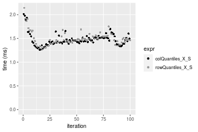
Figure: Benchmarking of colQuantiles_X_S() and rowQuantiles_X_S() on 10x10 data (original and transposed). Outliers are displayed as crosses. Times are in milliseconds.

100x100 matrix

> X <- data[["100x100"]]
> rows <- sample.int(nrow(X), size = nrow(X) * 0.7)
> cols <- sample.int(ncol(X), size = ncol(X) * 0.7)
> X_S <- X[rows, cols]
> gc()
           used  (Mb) gc trigger  (Mb) max used  (Mb)
Ncells  5268597 281.4    8529671 455.6  8529671 455.6
Vcells 10083645  77.0   31876688 243.2 60562128 462.1
> probs <- seq(from = 0, to = 1, by = 0.25)
> colStats <- microbenchmark(colQuantiles_X_S = colQuantiles(X_S, probs = probs, na.rm = FALSE), `colQuantiles(X, rows, cols)` = colQuantiles(X, 
+     rows = rows, cols = cols, probs = probs, na.rm = FALSE), `colQuantiles(X[rows, cols])` = colQuantiles(X[rows, 
+     cols], probs = probs, na.rm = FALSE), unit = "ms")
> X <- t(X)
> X_S <- t(X_S)
> gc()
           used  (Mb) gc trigger  (Mb) max used  (Mb)
Ncells  5268591 281.4    8529671 455.6  8529671 455.6
Vcells 10093728  77.1   31876688 243.2 60562128 462.1
> rowStats <- microbenchmark(rowQuantiles_X_S = rowQuantiles(X_S, probs = probs, na.rm = FALSE), `rowQuantiles(X, cols, rows)` = rowQuantiles(X, 
+     rows = cols, cols = rows, probs = probs, na.rm = FALSE), `rowQuantiles(X[cols, rows])` = rowQuantiles(X[cols, 
+     rows], probs = probs, na.rm = FALSE), unit = "ms")

Table: Benchmarking of colQuantiles_X_S(), colQuantiles(X, rows, cols)() and colQuantiles(X[rows, cols])() on 100x100 data. The top panel shows times in milliseconds and the bottom panel shows relative times.

	expr	min	lq	mean	median	uq	max
1	colQuantiles_X_S	1.259280	1.393225	1.472565	1.441515	1.513841	2.013098
3	colQuantiles(X[rows, cols])	1.263399	1.407822	1.587726	1.452552	1.540334	11.213533
2	colQuantiles(X, rows, cols)	1.267753	1.408001	1.493309	1.462292	1.524339	2.465260

	expr	min	lq	mean	median	uq	max
1	colQuantiles_X_S	1.000000	1.000000	1.000000	1.000000	1.000000	1.000000
3	colQuantiles(X[rows, cols])	1.003271	1.010478	1.078204	1.007656	1.017501	5.570287
2	colQuantiles(X, rows, cols)	1.006728	1.010606	1.014087	1.014413	1.006935	1.224610

Table: Benchmarking of rowQuantiles_X_S(), rowQuantiles(X, cols, rows)() and rowQuantiles(X[cols, rows])() on 100x100 data (transposed). The top panel shows times in milliseconds and the bottom panel shows relative times.

	expr	min	lq	mean	median	uq	max
1	rowQuantiles_X_S	1.270278	1.413137	1.492121	1.464138	1.540313	2.143832
3	rowQuantiles(X[cols, rows])	1.282105	1.426494	1.484845	1.484630	1.549282	1.837942
2	rowQuantiles(X, cols, rows)	1.296294	1.440462	1.619187	1.485569	1.549843	12.371649

	expr	min	lq	mean	median	uq	max
1	rowQuantiles_X_S	1.000000	1.000000	1.0000000	1.000000	1.000000	1.0000000
3	rowQuantiles(X[cols, rows])	1.009311	1.009452	0.9951238	1.013997	1.005823	0.8573162
2	rowQuantiles(X, cols, rows)	1.020481	1.019336	1.0851580	1.014638	1.006187	5.7708109

Figure: Benchmarking of colQuantiles_X_S(), colQuantiles(X, rows, cols)() and colQuantiles(X[rows, cols])() on 100x100 data as well as rowQuantiles_X_S(), rowQuantiles(X, cols, rows)() and rowQuantiles(X[cols, rows])() on the same data transposed. Outliers are displayed as crosses. Times are in milliseconds.

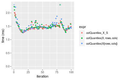
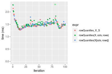Table: Benchmarking of colQuantiles_X_S() and rowQuantiles_X_S() on 100x100 data (original and transposed). The top panel shows times in milliseconds and the bottom panel shows relative times.

	expr	min	lq	mean	median	uq	max
1	colQuantiles_X_S	1.259280	1.393225	1.472565	1.441515	1.513841	2.013098
2	rowQuantiles_X_S	1.270278	1.413137	1.492121	1.464138	1.540313	2.143832

	expr	min	lq	mean	median	uq	max
1	colQuantiles_X_S	1.000000	1.000000	1.00000	1.000000	1.000000	1.000000
2	rowQuantiles_X_S	1.008734	1.014292	1.01328	1.015693	1.017487	1.064942

Figure: Benchmarking of colQuantiles_X_S() and rowQuantiles_X_S() on 100x100 data (original and transposed). Outliers are displayed as crosses. Times are in milliseconds.

1000x10 matrix

> X <- data[["1000x10"]]
> rows <- sample.int(nrow(X), size = nrow(X) * 0.7)
> cols <- sample.int(ncol(X), size = ncol(X) * 0.7)
> X_S <- X[rows, cols]
> gc()
           used  (Mb) gc trigger  (Mb) max used  (Mb)
Ncells  5269340 281.5    8529671 455.6  8529671 455.6
Vcells 10087697  77.0   31876688 243.2 60562128 462.1
> probs <- seq(from = 0, to = 1, by = 0.25)
> colStats <- microbenchmark(colQuantiles_X_S = colQuantiles(X_S, probs = probs, na.rm = FALSE), `colQuantiles(X, rows, cols)` = colQuantiles(X, 
+     rows = rows, cols = cols, probs = probs, na.rm = FALSE), `colQuantiles(X[rows, cols])` = colQuantiles(X[rows, 
+     cols], probs = probs, na.rm = FALSE), unit = "ms")
> X <- t(X)
> X_S <- t(X_S)
> gc()
           used  (Mb) gc trigger  (Mb) max used  (Mb)
Ncells  5269334 281.5    8529671 455.6  8529671 455.6
Vcells 10097780  77.1   31876688 243.2 60562128 462.1
> rowStats <- microbenchmark(rowQuantiles_X_S = rowQuantiles(X_S, probs = probs, na.rm = FALSE), `rowQuantiles(X, cols, rows)` = rowQuantiles(X, 
+     rows = cols, cols = rows, probs = probs, na.rm = FALSE), `rowQuantiles(X[cols, rows])` = rowQuantiles(X[cols, 
+     rows], probs = probs, na.rm = FALSE), unit = "ms")

Table: Benchmarking of colQuantiles_X_S(), colQuantiles(X, rows, cols)() and colQuantiles(X[rows, cols])() on 1000x10 data. The top panel shows times in milliseconds and the bottom panel shows relative times.

	expr	min	lq	mean	median	uq	max
1	colQuantiles_X_S	0.376902	0.3857895	0.4334700	0.4091225	0.4526740	0.657567
2	colQuantiles(X, rows, cols)	0.391405	0.4113425	0.4483459	0.4247020	0.4662810	0.671658
3	colQuantiles(X[rows, cols])	0.389880	0.4108325	0.4526213	0.4281940	0.4662545	0.831225

	expr	min	lq	mean	median	uq	max
1	colQuantiles_X_S	1.000000	1.000000	1.000000	1.000000	1.000000	1.000000
2	colQuantiles(X, rows, cols)	1.038479	1.066236	1.034318	1.038080	1.030059	1.021429
3	colQuantiles(X[rows, cols])	1.034433	1.064914	1.044181	1.046616	1.030001	1.264092

Table: Benchmarking of rowQuantiles_X_S(), rowQuantiles(X, cols, rows)() and rowQuantiles(X[cols, rows])() on 1000x10 data (transposed). The top panel shows times in milliseconds and the bottom panel shows relative times.

	expr	min	lq	mean	median	uq	max
1	rowQuantiles_X_S	0.396712	0.4071405	0.4485341	0.425961	0.4533000	0.675619
3	rowQuantiles(X[cols, rows])	0.412020	0.4235275	0.4663508	0.447727	0.4664785	0.871216
2	rowQuantiles(X, cols, rows)	0.412651	0.4342215	0.4690103	0.449217	0.4880695	0.659716

	expr	min	lq	mean	median	uq	max
1	rowQuantiles_X_S	1.000000	1.000000	1.000000	1.000000	1.000000	1.0000000
3	rowQuantiles(X[cols, rows])	1.038587	1.040249	1.039722	1.051099	1.029072	1.2895078
2	rowQuantiles(X, cols, rows)	1.040178	1.066515	1.045651	1.054596	1.076703	0.9764616

Figure: Benchmarking of colQuantiles_X_S(), colQuantiles(X, rows, cols)() and colQuantiles(X[rows, cols])() on 1000x10 data as well as rowQuantiles_X_S(), rowQuantiles(X, cols, rows)() and rowQuantiles(X[cols, rows])() on the same data transposed. Outliers are displayed as crosses. Times are in milliseconds.

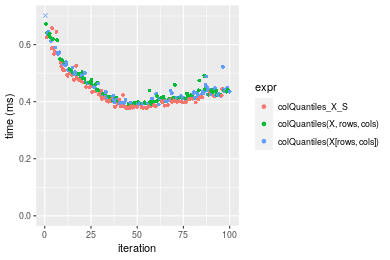
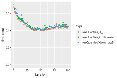Table: Benchmarking of colQuantiles_X_S() and rowQuantiles_X_S() on 1000x10 data (original and transposed). The top panel shows times in milliseconds and the bottom panel shows relative times.

	expr	min	lq	mean	median	uq	max
1	colQuantiles_X_S	376.902	385.7895	433.4700	409.1225	452.674	657.567
2	rowQuantiles_X_S	396.712	407.1405	448.5341	425.9610	453.300	675.619

	expr	min	lq	mean	median	uq	max
1	colQuantiles_X_S	1.00000	1.000000	1.000000	1.000000	1.000000	1.000000
2	rowQuantiles_X_S	1.05256	1.055344	1.034752	1.041158	1.001383	1.027453

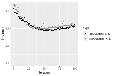
Figure: Benchmarking of colQuantiles_X_S() and rowQuantiles_X_S() on 1000x10 data (original and transposed). Outliers are displayed as crosses. Times are in milliseconds.

10x1000 matrix

> X <- data[["10x1000"]]
> rows <- sample.int(nrow(X), size = nrow(X) * 0.7)
> cols <- sample.int(ncol(X), size = ncol(X) * 0.7)
> X_S <- X[rows, cols]
> gc()
           used  (Mb) gc trigger  (Mb) max used  (Mb)
Ncells  5269545 281.5    8529671 455.6  8529671 455.6
Vcells 10088684  77.0   31876688 243.2 60562128 462.1
> probs <- seq(from = 0, to = 1, by = 0.25)
> colStats <- microbenchmark(colQuantiles_X_S = colQuantiles(X_S, probs = probs, na.rm = FALSE), `colQuantiles(X, rows, cols)` = colQuantiles(X, 
+     rows = rows, cols = cols, probs = probs, na.rm = FALSE), `colQuantiles(X[rows, cols])` = colQuantiles(X[rows, 
+     cols], probs = probs, na.rm = FALSE), unit = "ms")
> X <- t(X)
> X_S <- t(X_S)
> gc()
           used  (Mb) gc trigger  (Mb) max used  (Mb)
Ncells  5269539 281.5    8529671 455.6  8529671 455.6
Vcells 10098767  77.1   31876688 243.2 60562128 462.1
> rowStats <- microbenchmark(rowQuantiles_X_S = rowQuantiles(X_S, probs = probs, na.rm = FALSE), `rowQuantiles(X, cols, rows)` = rowQuantiles(X, 
+     rows = cols, cols = rows, probs = probs, na.rm = FALSE), `rowQuantiles(X[cols, rows])` = rowQuantiles(X[cols, 
+     rows], probs = probs, na.rm = FALSE), unit = "ms")

Table: Benchmarking of colQuantiles_X_S(), colQuantiles(X, rows, cols)() and colQuantiles(X[rows, cols])() on 10x1000 data. The top panel shows times in milliseconds and the bottom panel shows relative times.

	expr	min	lq	mean	median	uq	max
3	colQuantiles(X[rows, cols])	9.442057	10.70863	11.20262	10.88031	11.17366	17.73532
1	colQuantiles_X_S	9.827438	10.67614	10.99559	10.90096	11.14681	17.44323
2	colQuantiles(X, rows, cols)	9.605101	10.75428	11.30458	10.94825	11.16329	22.75870

	expr	min	lq	mean	median	uq	max
3	colQuantiles(X[rows, cols])	1.000000	1.0000000	1.0000000	1.000000	1.0000000	1.0000000
1	colQuantiles_X_S	1.040815	0.9969656	0.9815187	1.001898	0.9975973	0.9835305
2	colQuantiles(X, rows, cols)	1.017268	1.0042629	1.0091012	1.006244	0.9990723	1.2832416

Table: Benchmarking of rowQuantiles_X_S(), rowQuantiles(X, cols, rows)() and rowQuantiles(X[cols, rows])() on 10x1000 data (transposed). The top panel shows times in milliseconds and the bottom panel shows relative times.

	expr	min	lq	mean	median	uq	max
2	rowQuantiles(X, cols, rows)	9.386004	10.76202	11.16303	10.92739	11.19759	18.26512
1	rowQuantiles_X_S	9.806843	10.77164	11.23187	10.96238	11.18627	17.59954
3	rowQuantiles(X[cols, rows])	9.317670	10.81869	11.21185	10.99886	11.19615	17.79435

	expr	min	lq	mean	median	uq	max
2	rowQuantiles(X, cols, rows)	1.0000000	1.000000	1.000000	1.000000	1.0000000	1.0000000
1	rowQuantiles_X_S	1.0448369	1.000894	1.006166	1.003203	0.9989891	0.9635605
3	rowQuantiles(X[cols, rows])	0.9927196	1.005266	1.004373	1.006541	0.9998717	0.9742262

Figure: Benchmarking of colQuantiles_X_S(), colQuantiles(X, rows, cols)() and colQuantiles(X[rows, cols])() on 10x1000 data as well as rowQuantiles_X_S(), rowQuantiles(X, cols, rows)() and rowQuantiles(X[cols, rows])() on the same data transposed. Outliers are displayed as crosses. Times are in milliseconds.

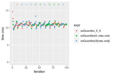
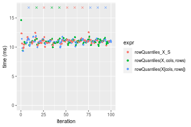Table: Benchmarking of colQuantiles_X_S() and rowQuantiles_X_S() on 10x1000 data (original and transposed). The top panel shows times in milliseconds and the bottom panel shows relative times.

	expr	min	lq	mean	median	uq	max
1	colQuantiles_X_S	9.827438	10.67614	10.99559	10.90096	11.14681	17.44323
2	rowQuantiles_X_S	9.806843	10.77164	11.23187	10.96238	11.18627	17.59954

	expr	min	lq	mean	median	uq	max
1	colQuantiles_X_S	1.0000000	1.000000	1.000000	1.000000	1.00000	1.000000
2	rowQuantiles_X_S	0.9979043	1.008945	1.021489	1.005635	1.00354	1.008961

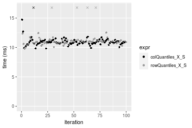
Figure: Benchmarking of colQuantiles_X_S() and rowQuantiles_X_S() on 10x1000 data (original and transposed). Outliers are displayed as crosses. Times are in milliseconds.

100x1000 matrix

> X <- data[["100x1000"]]
> rows <- sample.int(nrow(X), size = nrow(X) * 0.7)
> cols <- sample.int(ncol(X), size = ncol(X) * 0.7)
> X_S <- X[rows, cols]
> gc()
           used  (Mb) gc trigger  (Mb) max used  (Mb)
Ncells  5269767 281.5    8529671 455.6  8529671 455.6
Vcells 10133447  77.4   31876688 243.2 60562128 462.1
> probs <- seq(from = 0, to = 1, by = 0.25)
> colStats <- microbenchmark(colQuantiles_X_S = colQuantiles(X_S, probs = probs, na.rm = FALSE), `colQuantiles(X, rows, cols)` = colQuantiles(X, 
+     rows = rows, cols = cols, probs = probs, na.rm = FALSE), `colQuantiles(X[rows, cols])` = colQuantiles(X[rows, 
+     cols], probs = probs, na.rm = FALSE), unit = "ms")
> X <- t(X)
> X_S <- t(X_S)
> gc()
           used  (Mb) gc trigger  (Mb) max used  (Mb)
Ncells  5269749 281.5    8529671 455.6  8529671 455.6
Vcells 10233510  78.1   31876688 243.2 60562128 462.1
> rowStats <- microbenchmark(rowQuantiles_X_S = rowQuantiles(X_S, probs = probs, na.rm = FALSE), `rowQuantiles(X, cols, rows)` = rowQuantiles(X, 
+     rows = cols, cols = rows, probs = probs, na.rm = FALSE), `rowQuantiles(X[cols, rows])` = rowQuantiles(X[cols, 
+     rows], probs = probs, na.rm = FALSE), unit = "ms")

Table: Benchmarking of colQuantiles_X_S(), colQuantiles(X, rows, cols)() and colQuantiles(X[rows, cols])() on 100x1000 data. The top panel shows times in milliseconds and the bottom panel shows relative times.

	expr	min	lq	mean	median	uq	max
1	colQuantiles_X_S	12.22300	13.36760	14.12116	13.52681	13.79721	25.01684
2	colQuantiles(X, rows, cols)	12.28700	13.54403	14.38803	13.70976	13.98496	25.88454
3	colQuantiles(X[rows, cols])	11.75371	13.51295	13.68049	13.73721	13.94468	14.99997

	expr	min	lq	mean	median	uq	max
1	colQuantiles_X_S	1.0000000	1.000000	1.0000000	1.000000	1.000000	1.0000000
2	colQuantiles(X, rows, cols)	1.0052363	1.013198	1.0188987	1.013524	1.013608	1.0346847
3	colQuantiles(X[rows, cols])	0.9616057	1.010873	0.9687936	1.015554	1.010689	0.5995949

Table: Benchmarking of rowQuantiles_X_S(), rowQuantiles(X, cols, rows)() and rowQuantiles(X[cols, rows])() on 100x1000 data (transposed). The top panel shows times in milliseconds and the bottom panel shows relative times.

	expr	min	lq	mean	median	uq	max
1	rowQuantiles_X_S	12.49744	13.70006	14.27917	13.92902	14.22438	25.77719
3	rowQuantiles(X[cols, rows])	12.27313	13.94419	14.79305	14.13867	14.32470	37.72975
2	rowQuantiles(X, cols, rows)	12.80339	13.95292	14.49924	14.15657	14.35943	25.69399

	expr	min	lq	mean	median	uq	max
1	rowQuantiles_X_S	1.0000000	1.000000	1.000000	1.000000	1.000000	1.000000
3	rowQuantiles(X[cols, rows])	0.9820518	1.017820	1.035988	1.015051	1.007052	1.463687
2	rowQuantiles(X, cols, rows)	1.0244810	1.018457	1.015412	1.016337	1.009494	0.996772

Figure: Benchmarking of colQuantiles_X_S(), colQuantiles(X, rows, cols)() and colQuantiles(X[rows, cols])() on 100x1000 data as well as rowQuantiles_X_S(), rowQuantiles(X, cols, rows)() and rowQuantiles(X[cols, rows])() on the same data transposed. Outliers are displayed as crosses. Times are in milliseconds.

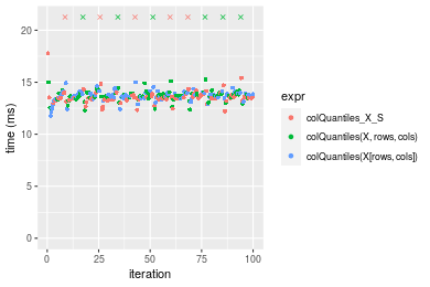
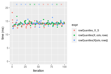Table: Benchmarking of colQuantiles_X_S() and rowQuantiles_X_S() on 100x1000 data (original and transposed). The top panel shows times in milliseconds and the bottom panel shows relative times.

	expr	min	lq	mean	median	uq	max
1	colQuantiles_X_S	12.22300	13.36760	14.12116	13.52681	13.79721	25.01684
2	rowQuantiles_X_S	12.49744	13.70006	14.27917	13.92902	14.22438	25.77719

	expr	min	lq	mean	median	uq	max
1	colQuantiles_X_S	1.000000	1.000000	1.000000	1.000000	1.000000	1.000000
2	rowQuantiles_X_S	1.022453	1.024871	1.011189	1.029734	1.030961	1.030394

Figure: Benchmarking of colQuantiles_X_S() and rowQuantiles_X_S() on 100x1000 data (original and transposed). Outliers are displayed as crosses. Times are in milliseconds.

1000x100 matrix

> X <- data[["1000x100"]]
> rows <- sample.int(nrow(X), size = nrow(X) * 0.7)
> cols <- sample.int(ncol(X), size = ncol(X) * 0.7)
> X_S <- X[rows, cols]
> gc()
           used  (Mb) gc trigger  (Mb) max used  (Mb)
Ncells  5269980 281.5    8529671 455.6  8529671 455.6
Vcells 10134275  77.4   31876688 243.2 60562128 462.1
> probs <- seq(from = 0, to = 1, by = 0.25)
> colStats <- microbenchmark(colQuantiles_X_S = colQuantiles(X_S, probs = probs, na.rm = FALSE), `colQuantiles(X, rows, cols)` = colQuantiles(X, 
+     rows = rows, cols = cols, probs = probs, na.rm = FALSE), `colQuantiles(X[rows, cols])` = colQuantiles(X[rows, 
+     cols], probs = probs, na.rm = FALSE), unit = "ms")
> X <- t(X)
> X_S <- t(X_S)
> gc()
           used  (Mb) gc trigger  (Mb) max used  (Mb)
Ncells  5269962 281.5    8529671 455.6  8529671 455.6
Vcells 10234338  78.1   31876688 243.2 60562128 462.1
> rowStats <- microbenchmark(rowQuantiles_X_S = rowQuantiles(X_S, probs = probs, na.rm = FALSE), `rowQuantiles(X, cols, rows)` = rowQuantiles(X, 
+     rows = cols, cols = rows, probs = probs, na.rm = FALSE), `rowQuantiles(X[cols, rows])` = rowQuantiles(X[cols, 
+     rows], probs = probs, na.rm = FALSE), unit = "ms")

Table: Benchmarking of colQuantiles_X_S(), colQuantiles(X, rows, cols)() and colQuantiles(X[rows, cols])() on 1000x100 data. The top panel shows times in milliseconds and the bottom panel shows relative times.

	expr	min	lq	mean	median	uq	max
1	colQuantiles_X_S	2.929666	3.283390	3.354438	3.318930	3.384416	4.841613
3	colQuantiles(X[rows, cols])	3.115852	3.411503	3.492563	3.454354	3.537214	4.350086
2	colQuantiles(X, rows, cols)	2.992192	3.412097	3.678507	3.462241	3.532310	13.599391

	expr	min	lq	mean	median	uq	max
1	colQuantiles_X_S	1.000000	1.000000	1.000000	1.000000	1.000000	1.0000000
3	colQuantiles(X[rows, cols])	1.063552	1.039019	1.041177	1.040803	1.045147	0.8984787
2	colQuantiles(X, rows, cols)	1.021342	1.039199	1.096609	1.043180	1.043699	2.8088554

Table: Benchmarking of rowQuantiles_X_S(), rowQuantiles(X, cols, rows)() and rowQuantiles(X[cols, rows])() on 1000x100 data (transposed). The top panel shows times in milliseconds and the bottom panel shows relative times.

	expr	min	lq	mean	median	uq	max
1	rowQuantiles_X_S	3.194023	3.519172	3.576079	3.554039	3.629571	4.048947
2	rowQuantiles(X, cols, rows)	3.286063	3.665307	3.776926	3.728198	3.805614	5.454258
3	rowQuantiles(X[cols, rows])	3.289315	3.676176	3.952174	3.743796	3.841694	13.341035

	expr	min	lq	mean	median	uq	max
1	rowQuantiles_X_S	1.000000	1.000000	1.000000	1.000000	1.000000	1.000000
2	rowQuantiles(X, cols, rows)	1.028816	1.041525	1.056164	1.049003	1.048502	1.347081
3	rowQuantiles(X[cols, rows])	1.029834	1.044614	1.105169	1.053392	1.058443	3.294939

Figure: Benchmarking of colQuantiles_X_S(), colQuantiles(X, rows, cols)() and colQuantiles(X[rows, cols])() on 1000x100 data as well as rowQuantiles_X_S(), rowQuantiles(X, cols, rows)() and rowQuantiles(X[cols, rows])() on the same data transposed. Outliers are displayed as crosses. Times are in milliseconds.

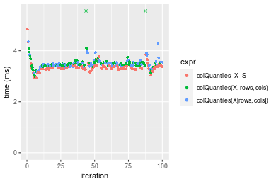
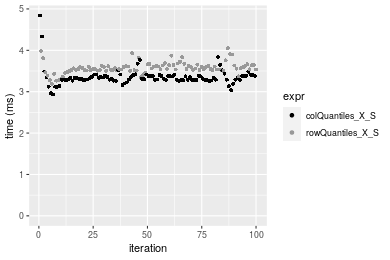
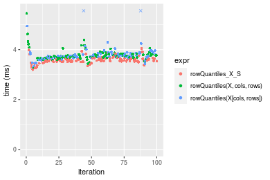Table: Benchmarking of colQuantiles_X_S() and rowQuantiles_X_S() on 1000x100 data (original and transposed). The top panel shows times in milliseconds and the bottom panel shows relative times.

	expr	min	lq	mean	median	uq	max
1	colQuantiles_X_S	2.929666	3.283390	3.354438	3.318930	3.384416	4.841613
2	rowQuantiles_X_S	3.194023	3.519172	3.576079	3.554039	3.629571	4.048947

	expr	min	lq	mean	median	uq	max
1	colQuantiles_X_S	1.000000	1.000000	1.000000	1.000000	1.000000	1.0000000
2	rowQuantiles_X_S	1.090234	1.071811	1.066074	1.070839	1.072436	0.8362806

Figure: Benchmarking of colQuantiles_X_S() and rowQuantiles_X_S() on 1000x100 data (original and transposed). Outliers are displayed as crosses. Times are in milliseconds.

Appendix

Session information

R version 4.1.1 Patched (2021-08-10 r80727)
Platform: x86_64-pc-linux-gnu (64-bit)
Running under: Ubuntu 18.04.5 LTS

Matrix products: default
BLAS:   /home/hb/software/R-devel/R-4-1-branch/lib/R/lib/libRblas.so
LAPACK: /home/hb/software/R-devel/R-4-1-branch/lib/R/lib/libRlapack.so

locale:
 [1] LC_CTYPE=en_US.UTF-8       LC_NUMERIC=C              
 [3] LC_TIME=en_US.UTF-8        LC_COLLATE=en_US.UTF-8    
 [5] LC_MONETARY=en_US.UTF-8    LC_MESSAGES=en_US.UTF-8   
 [7] LC_PAPER=en_US.UTF-8       LC_NAME=C                 
 [9] LC_ADDRESS=C               LC_TELEPHONE=C            
[11] LC_MEASUREMENT=en_US.UTF-8 LC_IDENTIFICATION=C       

attached base packages:
[1] stats     graphics  grDevices utils     datasets  methods   base     

other attached packages:
[1] microbenchmark_1.4-7   matrixStats_0.60.1     ggplot2_3.3.5         
[4] knitr_1.33             R.devices_2.17.0       R.utils_2.10.1        
[7] R.oo_1.24.0            R.methodsS3_1.8.1-9001 history_0.0.1-9000    

loaded via a namespace (and not attached):
 [1] Biobase_2.52.0          httr_1.4.2              splines_4.1.1          
 [4] bit64_4.0.5             network_1.17.1          assertthat_0.2.1       
 [7] highr_0.9               stats4_4.1.1            blob_1.2.2             
[10] GenomeInfoDbData_1.2.6  robustbase_0.93-8       pillar_1.6.2           
[13] RSQLite_2.2.8           lattice_0.20-44         glue_1.4.2             
[16] digest_0.6.27           XVector_0.32.0          colorspace_2.0-2       
[19] Matrix_1.3-4            XML_3.99-0.7            pkgconfig_2.0.3        
[22] zlibbioc_1.38.0         genefilter_1.74.0       purrr_0.3.4            
[25] ergm_4.1.2              xtable_1.8-4            scales_1.1.1           
[28] tibble_3.1.4            annotate_1.70.0         KEGGREST_1.32.0        
[31] farver_2.1.0            generics_0.1.0          IRanges_2.26.0         
[34] ellipsis_0.3.2          cachem_1.0.6            withr_2.4.2            
[37] BiocGenerics_0.38.0     mime_0.11               survival_3.2-13        
[40] magrittr_2.0.1          crayon_1.4.1            statnet.common_4.5.0   
[43] memoise_2.0.0           laeken_0.5.1            fansi_0.5.0            
[46] R.cache_0.15.0          MASS_7.3-54             R.rsp_0.44.0           
[49] progressr_0.8.0         tools_4.1.1             lifecycle_1.0.0        
[52] S4Vectors_0.30.0        trust_0.1-8             munsell_0.5.0          
[55] tabby_0.0.1-9001        AnnotationDbi_1.54.1    Biostrings_2.60.2      
[58] compiler_4.1.1          GenomeInfoDb_1.28.1     rlang_0.4.11           
[61] grid_4.1.1              RCurl_1.98-1.4          cwhmisc_6.6            
[64] rappdirs_0.3.3          startup_0.15.0          labeling_0.4.2         
[67] bitops_1.0-7            base64enc_0.1-3         boot_1.3-28            
[70] gtable_0.3.0            DBI_1.1.1               markdown_1.1           
[73] R6_2.5.1                lpSolveAPI_5.5.2.0-17.7 rle_0.9.2              
[76] dplyr_1.0.7             fastmap_1.1.0           bit_4.0.4              
[79] utf8_1.2.2              parallel_4.1.1          Rcpp_1.0.7             
[82] vctrs_0.3.8             png_0.1-7               DEoptimR_1.0-9         
[85] tidyselect_1.1.1        xfun_0.25               coda_0.19-4            

Total processing time was 30.55 secs.

Reproducibility

To reproduce this report, do:

html <- matrixStats:::benchmark('colRowQuantiles_subset')