matrixStats.benchmarks
colQuantiles() and rowQuantiles() benchmarks
This report benchmark the performance of colQuantiles() and rowQuantiles() against alternative methods.
Alternative methods
- apply() + quantile()
Data
> rmatrix <- function(nrow, ncol, mode = c("logical", "double", "integer", "index"), range = c(-100,
+     +100), na_prob = 0) {
+     mode <- match.arg(mode)
+     n <- nrow * ncol
+     if (mode == "logical") {
+         x <- sample(c(FALSE, TRUE), size = n, replace = TRUE)
+     }     else if (mode == "index") {
+         x <- seq_len(n)
+         mode <- "integer"
+     }     else {
+         x <- runif(n, min = range[1], max = range[2])
+     }
+     storage.mode(x) <- mode
+     if (na_prob > 0)
+         x[sample(n, size = na_prob * n)] <- NA
+     dim(x) <- c(nrow, ncol)
+     x
+ }
> rmatrices <- function(scale = 10, seed = 1, ...) {
+     set.seed(seed)
+     data <- list()
+     data[[1]] <- rmatrix(nrow = scale * 1, ncol = scale * 1, ...)
+     data[[2]] <- rmatrix(nrow = scale * 10, ncol = scale * 10, ...)
+     data[[3]] <- rmatrix(nrow = scale * 100, ncol = scale * 1, ...)
+     data[[4]] <- t(data[[3]])
+     data[[5]] <- rmatrix(nrow = scale * 10, ncol = scale * 100, ...)
+     data[[6]] <- t(data[[5]])
+     names(data) <- sapply(data, FUN = function(x) paste(dim(x), collapse = "x"))
+     data
+ }
> data <- rmatrices(mode = "double")
Results
10x10 matrix
> X <- data[["10x10"]]
> gc()
           used  (Mb) gc trigger  (Mb) max used  (Mb)
Ncells  5282673 282.2    8529671 455.6  8529671 455.6
Vcells 10520122  80.3   31876688 243.2 60562128 462.1
> probs <- seq(from = 0, to = 1, by = 0.25)
> colStats <- microbenchmark(colQuantiles = colQuantiles(X, probs = probs, na.rm = FALSE), `apply+quantile` = apply(X,
+     MARGIN = 2L, FUN = quantile, probs = probs, na.rm = FALSE), unit = "ms")
> X <- t(X)
> gc()
           used  (Mb) gc trigger  (Mb) max used  (Mb)
Ncells  5272450 281.6    8529671 455.6  8529671 455.6
Vcells 10486542  80.1   31876688 243.2 60562128 462.1
> rowStats <- microbenchmark(rowQuantiles = rowQuantiles(X, probs = probs, na.rm = FALSE), `apply+quantile` = apply(X,
+     MARGIN = 1L, FUN = quantile, probs = probs, na.rm = FALSE), unit = "ms")
Table: Benchmarking of colQuantiles() and apply+quantile() on 10x10 data. The top panel shows times in milliseconds and the bottom panel shows relative times.
| expr | min | lq | mean | median | uq | max | |
|---|---|---|---|---|---|---|---|
| 1 | colQuantiles | 0.240633 | 0.2628575 | 0.2890274 | 0.277496 | 0.3025895 | 0.479952 |
| 2 | apply+quantile | 1.060257 | 1.1672905 | 1.2570903 | 1.212705 | 1.2817150 | 2.025870 |
| expr | min | lq | mean | median | uq | max | |
|---|---|---|---|---|---|---|---|
| 1 | colQuantiles | 1.000000 | 1.000000 | 1.000000 | 1.000000 | 1.000000 | 1.000000 |
| 2 | apply+quantile | 4.406116 | 4.440773 | 4.349382 | 4.370173 | 4.235821 | 4.220985 |
Table: Benchmarking of rowQuantiles() and apply+quantile() on 10x10 data (transposed). The top panel shows times in milliseconds and the bottom panel shows relative times.
| expr | min | lq | mean | median | uq | max | |
|---|---|---|---|---|---|---|---|
| 1 | rowQuantiles | 0.235269 | 0.2596625 | 0.2863194 | 0.2733315 | 0.302111 | 0.468712 |
| 2 | apply+quantile | 1.069531 | 1.1232670 | 1.2350757 | 1.1880585 | 1.277098 | 2.041848 |
| expr | min | lq | mean | median | uq | max | |
|---|---|---|---|---|---|---|---|
| 1 | rowQuantiles | 1.000000 | 1.000000 | 1.000000 | 1.000000 | 1.000000 | 1.000000 |
| 2 | apply+quantile | 4.545992 | 4.325873 | 4.313629 | 4.346585 | 4.227248 | 4.356296 |
Figure: Benchmarking of colQuantiles() and apply+quantile() on 10x10 data as well as rowQuantiles() and apply+quantile() on the same data transposed. Outliers are displayed as crosses. Times are in milliseconds.
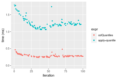
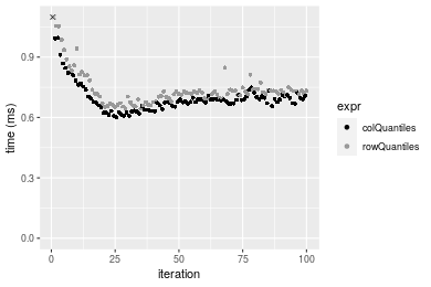
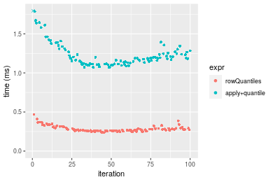 Table: Benchmarking of colQuantiles() and rowQuantiles() on 10x10 data (original and transposed). The top panel shows times in milliseconds and the bottom panel shows relative times.
| expr | min | lq | mean | median | uq | max | |
|---|---|---|---|---|---|---|---|
| 2 | rowQuantiles | 235.269 | 259.6625 | 286.3194 | 273.3315 | 302.1110 | 468.712 |
| 1 | colQuantiles | 240.633 | 262.8575 | 289.0274 | 277.4960 | 302.5895 | 479.952 |
| expr | min | lq | mean | median | uq | max | |
|---|---|---|---|---|---|---|---|
| 2 | rowQuantiles | 1.000000 | 1.000000 | 1.000000 | 1.000000 | 1.000000 | 1.000000 |
| 1 | colQuantiles | 1.022799 | 1.012304 | 1.009458 | 1.015236 | 1.001584 | 1.023981 |
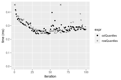
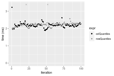
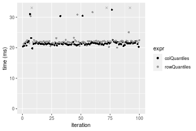
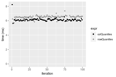
Figure: Benchmarking of colQuantiles() and rowQuantiles() on 10x10 data (original and transposed). Outliers are displayed as crosses. Times are in milliseconds.
100x100 matrix
> X <- data[["100x100"]]
> gc()
           used  (Mb) gc trigger  (Mb) max used  (Mb)
Ncells  5271016 281.6    8529671 455.6  8529671 455.6
Vcells 10102985  77.1   31876688 243.2 60562128 462.1
> probs <- seq(from = 0, to = 1, by = 0.25)
> colStats <- microbenchmark(colQuantiles = colQuantiles(X, probs = probs, na.rm = FALSE), `apply+quantile` = apply(X,
+     MARGIN = 2L, FUN = quantile, probs = probs, na.rm = FALSE), unit = "ms")
> X <- t(X)
> gc()
           used  (Mb) gc trigger  (Mb) max used  (Mb)
Ncells  5271004 281.6    8529671 455.6  8529671 455.6
Vcells 10113018  77.2   31876688 243.2 60562128 462.1
> rowStats <- microbenchmark(rowQuantiles = rowQuantiles(X, probs = probs, na.rm = FALSE), `apply+quantile` = apply(X,
+     MARGIN = 1L, FUN = quantile, probs = probs, na.rm = FALSE), unit = "ms")
Table: Benchmarking of colQuantiles() and apply+quantile() on 100x100 data. The top panel shows times in milliseconds and the bottom panel shows relative times.
| expr | min | lq | mean | median | uq | max | |
|---|---|---|---|---|---|---|---|
| 1 | colQuantiles | 1.888284 | 2.136058 | 2.195115 | 2.186279 | 2.243244 | 3.22735 |
| 2 | apply+quantile | 10.923141 | 12.262892 | 12.932966 | 12.499504 | 12.717576 | 33.25679 |
| expr | min | lq | mean | median | uq | max | |
|---|---|---|---|---|---|---|---|
| 1 | colQuantiles | 1.000000 | 1.000000 | 1.000000 | 1.00000 | 1.000000 | 1.00000 |
| 2 | apply+quantile | 5.784692 | 5.740897 | 5.891703 | 5.71725 | 5.669279 | 10.30467 |
Table: Benchmarking of rowQuantiles() and apply+quantile() on 100x100 data (transposed). The top panel shows times in milliseconds and the bottom panel shows relative times.
| expr | min | lq | mean | median | uq | max | |
|---|---|---|---|---|---|---|---|
| 1 | rowQuantiles | 1.947457 | 2.172823 | 2.370571 | 2.23365 | 2.274193 | 10.16345 |
| 2 | apply+quantile | 10.936896 | 12.217553 | 12.536485 | 12.40464 | 12.653492 | 21.03754 |
| expr | min | lq | mean | median | uq | max | |
|---|---|---|---|---|---|---|---|
| 1 | rowQuantiles | 1.000000 | 1.000000 | 1.000000 | 1.000000 | 1.000000 | 1.00000 |
| 2 | apply+quantile | 5.615988 | 5.622895 | 5.288382 | 5.553526 | 5.563948 | 2.06992 |
Figure: Benchmarking of colQuantiles() and apply+quantile() on 100x100 data as well as rowQuantiles() and apply+quantile() on the same data transposed. Outliers are displayed as crosses. Times are in milliseconds.
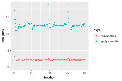
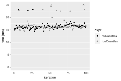
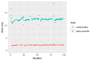 Table: Benchmarking of colQuantiles() and rowQuantiles() on 100x100 data (original and transposed). The top panel shows times in milliseconds and the bottom panel shows relative times.
| expr | min | lq | mean | median | uq | max | |
|---|---|---|---|---|---|---|---|
| 1 | colQuantiles | 1.888284 | 2.136058 | 2.195115 | 2.186279 | 2.243244 | 3.22735 |
| 2 | rowQuantiles | 1.947457 | 2.172823 | 2.370571 | 2.233650 | 2.274193 | 10.16345 |
| expr | min | lq | mean | median | uq | max | |
|---|---|---|---|---|---|---|---|
| 1 | colQuantiles | 1.000000 | 1.000000 | 1.00000 | 1.000000 | 1.000000 | 1.000000 |
| 2 | rowQuantiles | 1.031337 | 1.017211 | 1.07993 | 1.021668 | 1.013796 | 3.149164 |
Figure: Benchmarking of colQuantiles() and rowQuantiles() on 100x100 data (original and transposed). Outliers are displayed as crosses. Times are in milliseconds.
1000x10 matrix
> X <- data[["1000x10"]]
> gc()
           used  (Mb) gc trigger  (Mb) max used  (Mb)
Ncells  5271758 281.6    8529671 455.6  8529671 455.6
Vcells 10106514  77.2   31876688 243.2 60562128 462.1
> probs <- seq(from = 0, to = 1, by = 0.25)
> colStats <- microbenchmark(colQuantiles = colQuantiles(X, probs = probs, na.rm = FALSE), `apply+quantile` = apply(X,
+     MARGIN = 2L, FUN = quantile, probs = probs, na.rm = FALSE), unit = "ms")
> X <- t(X)
> gc()
           used  (Mb) gc trigger  (Mb) max used  (Mb)
Ncells  5271734 281.6    8529671 455.6  8529671 455.6
Vcells 10116527  77.2   31876688 243.2 60562128 462.1
> rowStats <- microbenchmark(rowQuantiles = rowQuantiles(X, probs = probs, na.rm = FALSE), `apply+quantile` = apply(X,
+     MARGIN = 1L, FUN = quantile, probs = probs, na.rm = FALSE), unit = "ms")
Table: Benchmarking of colQuantiles() and apply+quantile() on 1000x10 data. The top panel shows times in milliseconds and the bottom panel shows relative times.
| expr | min | lq | mean | median | uq | max | |
|---|---|---|---|---|---|---|---|
| 1 | colQuantiles | 0.601190 | 0.6562685 | 0.6981146 | 0.6862355 | 0.705663 | 1.156208 |
| 2 | apply+quantile | 1.503947 | 1.6398185 | 1.7177534 | 1.7044685 | 1.746963 | 2.498938 |
| expr | min | lq | mean | median | uq | max | |
|---|---|---|---|---|---|---|---|
| 1 | colQuantiles | 1.000000 | 1.000000 | 1.000000 | 1.000000 | 1.000000 | 1.000000 |
| 2 | apply+quantile | 2.501617 | 2.498701 | 2.460561 | 2.483795 | 2.475634 | 2.161322 |
Table: Benchmarking of rowQuantiles() and apply+quantile() on 1000x10 data (transposed). The top panel shows times in milliseconds and the bottom panel shows relative times.
| expr | min | lq | mean | median | uq | max | |
|---|---|---|---|---|---|---|---|
| 1 | rowQuantiles | 0.643236 | 0.694242 | 0.7400125 | 0.7194075 | 0.7373645 | 1.230742 |
| 2 | apply+quantile | 1.527078 | 1.654772 | 1.7342194 | 1.7038935 | 1.7511335 | 2.642374 |
| expr | min | lq | mean | median | uq | max | |
|---|---|---|---|---|---|---|---|
| 1 | rowQuantiles | 1.000000 | 1.000000 | 1.0000 | 1.000000 | 1.000000 | 1.000000 |
| 2 | apply+quantile | 2.374056 | 2.383567 | 2.3435 | 2.368468 | 2.374855 | 2.146976 |
Figure: Benchmarking of colQuantiles() and apply+quantile() on 1000x10 data as well as rowQuantiles() and apply+quantile() on the same data transposed. Outliers are displayed as crosses. Times are in milliseconds.
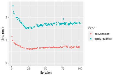
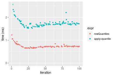 Table: Benchmarking of colQuantiles() and rowQuantiles() on 1000x10 data (original and transposed). The top panel shows times in milliseconds and the bottom panel shows relative times.
| expr | min | lq | mean | median | uq | max | |
|---|---|---|---|---|---|---|---|
| 1 | colQuantiles | 601.190 | 656.2685 | 698.1146 | 686.2355 | 705.6630 | 1156.208 |
| 2 | rowQuantiles | 643.236 | 694.2420 | 740.0125 | 719.4075 | 737.3645 | 1230.742 |
| expr | min | lq | mean | median | uq | max | |
|---|---|---|---|---|---|---|---|
| 1 | colQuantiles | 1.000000 | 1.000000 | 1.000000 | 1.000000 | 1.000000 | 1.000000 |
| 2 | rowQuantiles | 1.069938 | 1.057863 | 1.060016 | 1.048339 | 1.044924 | 1.064464 |
Figure: Benchmarking of colQuantiles() and rowQuantiles() on 1000x10 data (original and transposed). Outliers are displayed as crosses. Times are in milliseconds.
10x1000 matrix
> X <- data[["10x1000"]]
> gc()
           used  (Mb) gc trigger  (Mb) max used  (Mb)
Ncells  5271934 281.6    8529671 455.6  8529671 455.6
Vcells 10107214  77.2   31876688 243.2 60562128 462.1
> probs <- seq(from = 0, to = 1, by = 0.25)
> colStats <- microbenchmark(colQuantiles = colQuantiles(X, probs = probs, na.rm = FALSE), `apply+quantile` = apply(X,
+     MARGIN = 2L, FUN = quantile, probs = probs, na.rm = FALSE), unit = "ms")
> X <- t(X)
> gc()
           used  (Mb) gc trigger  (Mb) max used  (Mb)
Ncells  5271922 281.6    8529671 455.6  8529671 455.6
Vcells 10117247  77.2   31876688 243.2 60562128 462.1
> rowStats <- microbenchmark(rowQuantiles = rowQuantiles(X, probs = probs, na.rm = FALSE), `apply+quantile` = apply(X,
+     MARGIN = 1L, FUN = quantile, probs = probs, na.rm = FALSE), unit = "ms")
Table: Benchmarking of colQuantiles() and apply+quantile() on 10x1000 data. The top panel shows times in milliseconds and the bottom panel shows relative times.
| expr | min | lq | mean | median | uq | max | |
|---|---|---|---|---|---|---|---|
| 1 | colQuantiles | 14.45429 | 15.83936 | 16.89861 | 16.25864 | 16.82524 | 46.84812 |
| 2 | apply+quantile | 112.81877 | 116.21819 | 123.35627 | 119.25667 | 127.25195 | 161.59093 |
| expr | min | lq | mean | median | uq | max | |
|---|---|---|---|---|---|---|---|
| 1 | colQuantiles | 1.000000 | 1.000000 | 1.000000 | 1.000000 | 1.000000 | 1.000000 |
| 2 | apply+quantile | 7.805208 | 7.337304 | 7.299786 | 7.334974 | 7.563158 | 3.449251 |
Table: Benchmarking of rowQuantiles() and apply+quantile() on 10x1000 data (transposed). The top panel shows times in milliseconds and the bottom panel shows relative times.
| expr | min | lq | mean | median | uq | max | |
|---|---|---|---|---|---|---|---|
| 1 | rowQuantiles | 14.45924 | 15.9970 | 20.28669 | 16.20631 | 16.56712 | 381.9050 |
| 2 | apply+quantile | 110.53220 | 118.0066 | 121.22556 | 119.13909 | 125.02020 | 144.3018 |
| expr | min | lq | mean | median | uq | max | |
|---|---|---|---|---|---|---|---|
| 1 | rowQuantiles | 1.000000 | 1.000000 | 1.00000 | 1.000000 | 1.000000 | 1.0000000 |
| 2 | apply+quantile | 7.644397 | 7.376794 | 5.97562 | 7.351401 | 7.546282 | 0.3778473 |
Figure: Benchmarking of colQuantiles() and apply+quantile() on 10x1000 data as well as rowQuantiles() and apply+quantile() on the same data transposed. Outliers are displayed as crosses. Times are in milliseconds.
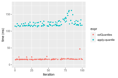
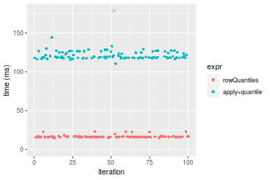 Table: Benchmarking of colQuantiles() and rowQuantiles() on 10x1000 data (original and transposed). The top panel shows times in milliseconds and the bottom panel shows relative times.
| expr | min | lq | mean | median | uq | max | |
|---|---|---|---|---|---|---|---|
| 2 | rowQuantiles | 14.45924 | 15.99700 | 20.28669 | 16.20631 | 16.56712 | 381.90503 |
| 1 | colQuantiles | 14.45429 | 15.83936 | 16.89861 | 16.25864 | 16.82524 | 46.84812 |
| expr | min | lq | mean | median | uq | max | |
|---|---|---|---|---|---|---|---|
| 2 | rowQuantiles | 1.0000000 | 1.0000000 | 1.0000000 | 1.000000 | 1.00000 | 1.0000000 |
| 1 | colQuantiles | 0.9996576 | 0.9901455 | 0.8329901 | 1.003229 | 1.01558 | 0.1226696 |
Figure: Benchmarking of colQuantiles() and rowQuantiles() on 10x1000 data (original and transposed). Outliers are displayed as crosses. Times are in milliseconds.
100x1000 matrix
> X <- data[["100x1000"]]
> gc()
           used  (Mb) gc trigger  (Mb) max used  (Mb)
Ncells  5272118 281.6    8529671 455.6  8529671 455.6
Vcells 10107704  77.2   31876688 243.2 60562128 462.1
> probs <- seq(from = 0, to = 1, by = 0.25)
> colStats <- microbenchmark(colQuantiles = colQuantiles(X, probs = probs, na.rm = FALSE), `apply+quantile` = apply(X,
+     MARGIN = 2L, FUN = quantile, probs = probs, na.rm = FALSE), unit = "ms")
> X <- t(X)
> gc()
           used  (Mb) gc trigger  (Mb) max used  (Mb)
Ncells  5272106 281.6    8529671 455.6  8529671 455.6
Vcells 10207737  77.9   31876688 243.2 60562128 462.1
> rowStats <- microbenchmark(rowQuantiles = rowQuantiles(X, probs = probs, na.rm = FALSE), `apply+quantile` = apply(X,
+     MARGIN = 1L, FUN = quantile, probs = probs, na.rm = FALSE), unit = "ms")
Table: Benchmarking of colQuantiles() and apply+quantile() on 100x1000 data. The top panel shows times in milliseconds and the bottom panel shows relative times.
| expr | min | lq | mean | median | uq | max | |
|---|---|---|---|---|---|---|---|
| 1 | colQuantiles | 19.78046 | 21.08175 | 21.71354 | 21.32056 | 21.61416 | 32.44358 |
| 2 | apply+quantile | 124.22724 | 127.17620 | 131.48661 | 128.56766 | 136.34522 | 150.63818 |
| expr | min | lq | mean | median | uq | max | |
|---|---|---|---|---|---|---|---|
| 1 | colQuantiles | 1.000000 | 1.000000 | 1.000000 | 1.000000 | 1.000000 | 1.000000 |
| 2 | apply+quantile | 6.280301 | 6.032525 | 6.055512 | 6.030219 | 6.308144 | 4.643082 |
Table: Benchmarking of rowQuantiles() and apply+quantile() on 100x1000 data (transposed). The top panel shows times in milliseconds and the bottom panel shows relative times.
| expr | min | lq | mean | median | uq | max | |
|---|---|---|---|---|---|---|---|
| 1 | rowQuantiles | 20.02987 | 21.71925 | 22.67224 | 21.97428 | 22.16405 | 44.66161 |
| 2 | apply+quantile | 123.55330 | 127.41662 | 131.43956 | 128.76763 | 136.82947 | 146.98970 |
| expr | min | lq | mean | median | uq | max | |
|---|---|---|---|---|---|---|---|
| 1 | rowQuantiles | 1.000000 | 1.000000 | 1.000000 | 1.000000 | 1.000000 | 1.000000 |
| 2 | apply+quantile | 6.168454 | 5.866531 | 5.797378 | 5.859925 | 6.173487 | 3.291187 |
Figure: Benchmarking of colQuantiles() and apply+quantile() on 100x1000 data as well as rowQuantiles() and apply+quantile() on the same data transposed. Outliers are displayed as crosses. Times are in milliseconds.
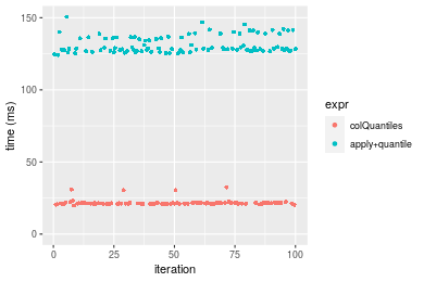
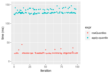 Table: Benchmarking of colQuantiles() and rowQuantiles() on 100x1000 data (original and transposed). The top panel shows times in milliseconds and the bottom panel shows relative times.
| expr | min | lq | mean | median | uq | max | |
|---|---|---|---|---|---|---|---|
| 1 | colQuantiles | 19.78046 | 21.08175 | 21.71354 | 21.32056 | 21.61416 | 32.44358 |
| 2 | rowQuantiles | 20.02987 | 21.71925 | 22.67224 | 21.97428 | 22.16405 | 44.66161 |
| expr | min | lq | mean | median | uq | max | |
|---|---|---|---|---|---|---|---|
| 1 | colQuantiles | 1.000000 | 1.000000 | 1.000000 | 1.000000 | 1.000000 | 1.000000 |
| 2 | rowQuantiles | 1.012609 | 1.030239 | 1.044152 | 1.030661 | 1.025441 | 1.376593 |
Figure: Benchmarking of colQuantiles() and rowQuantiles() on 100x1000 data (original and transposed). Outliers are displayed as crosses. Times are in milliseconds.
1000x100 matrix
> X <- data[["1000x100"]]
> gc()
           used  (Mb) gc trigger  (Mb) max used  (Mb)
Ncells  5272310 281.6    8529671 455.6  8529671 455.6
Vcells 10108335  77.2   31876688 243.2 60562128 462.1
> probs <- seq(from = 0, to = 1, by = 0.25)
> colStats <- microbenchmark(colQuantiles = colQuantiles(X, probs = probs, na.rm = FALSE), `apply+quantile` = apply(X,
+     MARGIN = 2L, FUN = quantile, probs = probs, na.rm = FALSE), unit = "ms")
> X <- t(X)
> gc()
           used  (Mb) gc trigger  (Mb) max used  (Mb)
Ncells  5272298 281.6    8529671 455.6  8529671 455.6
Vcells 10208368  77.9   31876688 243.2 60562128 462.1
> rowStats <- microbenchmark(rowQuantiles = rowQuantiles(X, probs = probs, na.rm = FALSE), `apply+quantile` = apply(X,
+     MARGIN = 1L, FUN = quantile, probs = probs, na.rm = FALSE), unit = "ms")
Table: Benchmarking of colQuantiles() and apply+quantile() on 1000x100 data. The top panel shows times in milliseconds and the bottom panel shows relative times.
| expr | min | lq | mean | median | uq | max | |
|---|---|---|---|---|---|---|---|
| 1 | colQuantiles | 5.636397 | 6.027108 | 6.135147 | 6.116474 | 6.188172 | 8.237741 |
| 2 | apply+quantile | 15.165356 | 17.037116 | 17.544969 | 17.240510 | 17.492228 | 28.635703 |
| expr | min | lq | mean | median | uq | max | |
|---|---|---|---|---|---|---|---|
| 1 | colQuantiles | 1.000000 | 1.000000 | 1.000000 | 1.000000 | 1.00000 | 1.00000 |
| 2 | apply+quantile | 2.690612 | 2.826748 | 2.859747 | 2.818701 | 2.82672 | 3.47616 |
Table: Benchmarking of rowQuantiles() and apply+quantile() on 1000x100 data (transposed). The top panel shows times in milliseconds and the bottom panel shows relative times.
| expr | min | lq | mean | median | uq | max | |
|---|---|---|---|---|---|---|---|
| 1 | rowQuantiles | 5.665498 | 6.479869 | 6.509218 | 6.53708 | 6.612499 | 7.358592 |
| 2 | apply+quantile | 15.444699 | 17.088696 | 17.574659 | 17.28185 | 17.448529 | 28.096502 |
| expr | min | lq | mean | median | uq | max | |
|---|---|---|---|---|---|---|---|
| 1 | rowQuantiles | 1.000000 | 1.000000 | 1.000000 | 1.000000 | 1.00000 | 1.00000 |
| 2 | apply+quantile | 2.726097 | 2.637198 | 2.699965 | 2.643664 | 2.63872 | 3.81819 |
Figure: Benchmarking of colQuantiles() and apply+quantile() on 1000x100 data as well as rowQuantiles() and apply+quantile() on the same data transposed. Outliers are displayed as crosses. Times are in milliseconds.
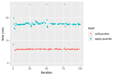
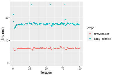 Table: Benchmarking of colQuantiles() and rowQuantiles() on 1000x100 data (original and transposed). The top panel shows times in milliseconds and the bottom panel shows relative times.
| expr | min | lq | mean | median | uq | max | |
|---|---|---|---|---|---|---|---|
| 1 | colQuantiles | 5.636397 | 6.027108 | 6.135147 | 6.116474 | 6.188172 | 8.237741 |
| 2 | rowQuantiles | 5.665498 | 6.479869 | 6.509218 | 6.537080 | 6.612499 | 7.358592 |
| expr | min | lq | mean | median | uq | max | |
|---|---|---|---|---|---|---|---|
| 1 | colQuantiles | 1.000000 | 1.000000 | 1.000000 | 1.000000 | 1.000000 | 1.0000000 |
| 2 | rowQuantiles | 1.005163 | 1.075121 | 1.060972 | 1.068766 | 1.068571 | 0.8932779 |
Figure: Benchmarking of colQuantiles() and rowQuantiles() on 1000x100 data (original and transposed). Outliers are displayed as crosses. Times are in milliseconds.
Appendix
Session information
R version 4.1.1 Patched (2021-08-10 r80727)
Platform: x86_64-pc-linux-gnu (64-bit)
Running under: Ubuntu 18.04.5 LTS

Matrix products: default
BLAS:   /home/hb/software/R-devel/R-4-1-branch/lib/R/lib/libRblas.so
LAPACK: /home/hb/software/R-devel/R-4-1-branch/lib/R/lib/libRlapack.so

locale:
 [1] LC_CTYPE=en_US.UTF-8       LC_NUMERIC=C
 [3] LC_TIME=en_US.UTF-8        LC_COLLATE=en_US.UTF-8
 [5] LC_MONETARY=en_US.UTF-8    LC_MESSAGES=en_US.UTF-8
 [7] LC_PAPER=en_US.UTF-8       LC_NAME=C
 [9] LC_ADDRESS=C               LC_TELEPHONE=C
[11] LC_MEASUREMENT=en_US.UTF-8 LC_IDENTIFICATION=C

attached base packages:
[1] stats     graphics  grDevices utils     datasets  methods   base

other attached packages:
[1] microbenchmark_1.4-7   matrixStats_0.60.1     ggplot2_3.3.5
[4] knitr_1.33             R.devices_2.17.0       R.utils_2.10.1
[7] R.oo_1.24.0            R.methodsS3_1.8.1-9001 history_0.0.1-9000

loaded via a namespace (and not attached):
 [1] Biobase_2.52.0          httr_1.4.2              splines_4.1.1
 [4] bit64_4.0.5             network_1.17.1          assertthat_0.2.1
 [7] highr_0.9               stats4_4.1.1            blob_1.2.2
[10] GenomeInfoDbData_1.2.6  robustbase_0.93-8       pillar_1.6.2
[13] RSQLite_2.2.8           lattice_0.20-44         glue_1.4.2
[16] digest_0.6.27           XVector_0.32.0          colorspace_2.0-2
[19] Matrix_1.3-4            XML_3.99-0.7            pkgconfig_2.0.3
[22] zlibbioc_1.38.0         genefilter_1.74.0       purrr_0.3.4
[25] ergm_4.1.2              xtable_1.8-4            scales_1.1.1
[28] tibble_3.1.4            annotate_1.70.0         KEGGREST_1.32.0
[31] farver_2.1.0            generics_0.1.0          IRanges_2.26.0
[34] ellipsis_0.3.2          cachem_1.0.6            withr_2.4.2
[37] BiocGenerics_0.38.0     mime_0.11               survival_3.2-13
[40] magrittr_2.0.1          crayon_1.4.1            statnet.common_4.5.0
[43] memoise_2.0.0           laeken_0.5.1            fansi_0.5.0
[46] R.cache_0.15.0          MASS_7.3-54             R.rsp_0.44.0
[49] progressr_0.8.0         tools_4.1.1             lifecycle_1.0.0
[52] S4Vectors_0.30.0        trust_0.1-8             munsell_0.5.0
[55] tabby_0.0.1-9001        AnnotationDbi_1.54.1    Biostrings_2.60.2
[58] compiler_4.1.1          GenomeInfoDb_1.28.1     rlang_0.4.11
[61] grid_4.1.1              RCurl_1.98-1.4          cwhmisc_6.6
[64] rappdirs_0.3.3          startup_0.15.0          labeling_0.4.2
[67] bitops_1.0-7            base64enc_0.1-3         boot_1.3-28
[70] gtable_0.3.0            DBI_1.1.1               markdown_1.1
[73] R6_2.5.1                lpSolveAPI_5.5.2.0-17.7 rle_0.9.2
[76] dplyr_1.0.7             fastmap_1.1.0           bit_4.0.4
[79] utf8_1.2.2              parallel_4.1.1          Rcpp_1.0.7
[82] vctrs_0.3.8             png_0.1-7               DEoptimR_1.0-9
[85] tidyselect_1.1.1        xfun_0.25               coda_0.19-4
Total processing time was 1.32 mins.
Reproducibility
To reproduce this report, do:
html <- matrixStats:::benchmark('colQuantiles')
Copyright Henrik Bengtsson. Last updated on 2021-08-25 19:06:31 (+0200 UTC). Powered by RSP.