matrixStats.benchmarks

colMedians() and rowMedians() benchmarks

This report benchmark the performance of colMedians() and rowMedians() against alternative methods.

Alternative methods

apply() + median()

Data type “integer”

Data

> rmatrix <- function(nrow, ncol, mode = c("logical", "double", "integer", "index"), range = c(-100, 
+     +100), na_prob = 0) {
+     mode <- match.arg(mode)
+     n <- nrow * ncol
+     if (mode == "logical") {
+         x <- sample(c(FALSE, TRUE), size = n, replace = TRUE)
+     }     else if (mode == "index") {
+         x <- seq_len(n)
+         mode <- "integer"
+     }     else {
+         x <- runif(n, min = range[1], max = range[2])
+     }
+     storage.mode(x) <- mode
+     if (na_prob > 0) 
+         x[sample(n, size = na_prob * n)] <- NA
+     dim(x) <- c(nrow, ncol)
+     x
+ }
> rmatrices <- function(scale = 10, seed = 1, ...) {
+     set.seed(seed)
+     data <- list()
+     data[[1]] <- rmatrix(nrow = scale * 1, ncol = scale * 1, ...)
+     data[[2]] <- rmatrix(nrow = scale * 10, ncol = scale * 10, ...)
+     data[[3]] <- rmatrix(nrow = scale * 100, ncol = scale * 1, ...)
+     data[[4]] <- t(data[[3]])
+     data[[5]] <- rmatrix(nrow = scale * 10, ncol = scale * 100, ...)
+     data[[6]] <- t(data[[5]])
+     names(data) <- sapply(data, FUN = function(x) paste(dim(x), collapse = "x"))
+     data
+ }
> data <- rmatrices(mode = mode)

Results

10x10 integer matrix

> X <- data[["10x10"]]
> gc()
           used  (Mb) gc trigger  (Mb) max used  (Mb)
Ncells  5252897 280.6    8529671 455.6  8529671 455.6
Vcells 10204002  77.9   31876688 243.2 60562128 462.1
> colStats <- microbenchmark(colMedians = colMedians(X, na.rm = FALSE), `apply+median` = apply(X, MARGIN = 2L, 
+     FUN = median, na.rm = FALSE), unit = "ms")
> X <- t(X)
> gc()
           used  (Mb) gc trigger  (Mb) max used  (Mb)
Ncells  5242876 280.0    8529671 455.6  8529671 455.6
Vcells 10171042  77.6   31876688 243.2 60562128 462.1
> rowStats <- microbenchmark(rowMedians = rowMedians(X, na.rm = FALSE), `apply+median` = apply(X, MARGIN = 1L, 
+     FUN = median, na.rm = FALSE), unit = "ms")

Table: Benchmarking of colMedians() and apply+median() on integer+10x10 data. The top panel shows times in milliseconds and the bottom panel shows relative times.

	expr	min	lq	mean	median	uq	max
1	colMedians	0.002002	0.0024270	0.0035696	0.0033185	0.0040520	0.016345
2	apply+median	0.310973	0.3230125	0.3543233	0.3410970	0.3817475	0.582277

	expr	min	lq	mean	median	uq	max
1	colMedians	1.0000	1.0000	1.00000	1.0000	1.00000	1.00000
2	apply+median	155.3312	133.0913	99.26191	102.7865	94.21212	35.62417

Table: Benchmarking of rowMedians() and apply+median() on integer+10x10 data (transposed). The top panel shows times in milliseconds and the bottom panel shows relative times.

	expr	min	lq	mean	median	uq	max
1	rowMedians	0.002156	0.0027635	0.0041715	0.0038790	0.004733	0.017459
2	apply+median	0.308591	0.3233260	0.3567586	0.3377955	0.385195	0.579707

	expr	min	lq	mean	median	uq	max
1	rowMedians	1.0000	1.0000	1.00000	1.00000	1.00000	1.00000
2	apply+median	143.1313	116.9987	85.52244	87.08314	81.38496	33.20391

Figure: Benchmarking of colMedians() and apply+median() on integer+10x10 data as well as rowMedians() and apply+median() on the same data transposed. Outliers are displayed as crosses. Times are in milliseconds.

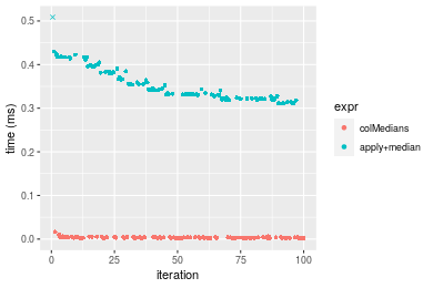
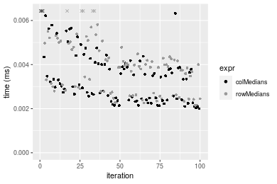
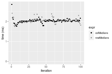
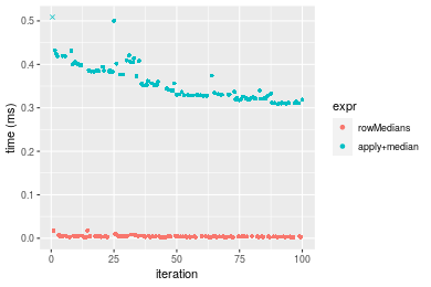Table: Benchmarking of colMedians() and rowMedians() on integer+10x10 data (original and transposed). The top panel shows times in milliseconds and the bottom panel shows relative times.

	expr	min	lq	mean	median	uq	max
1	colMedians	2.002	2.4270	3.56958	3.3185	4.052	16.345
2	rowMedians	2.156	2.7635	4.17152	3.8790	4.733	17.459

	expr	min	lq	mean	median	uq	max
1	colMedians	1.000000	1.000000	1.00000	1.000000	1.000000	1.000000
2	rowMedians	1.076923	1.138648	1.16863	1.168902	1.168065	1.068155

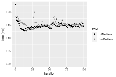
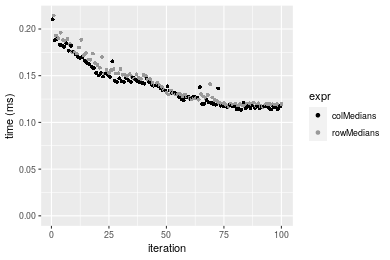
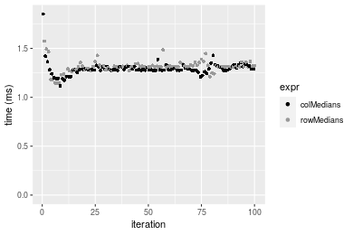
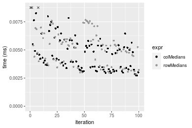
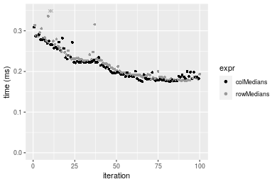
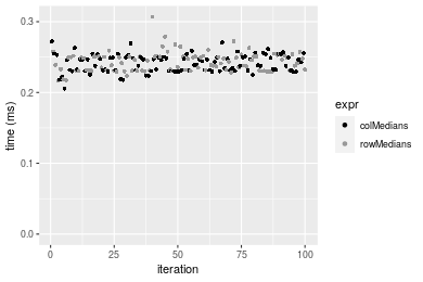
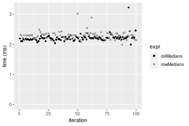
Figure: Benchmarking of colMedians() and rowMedians() on integer+10x10 data (original and transposed). Outliers are displayed as crosses. Times are in milliseconds.

100x100 integer matrix

> X <- data[["100x100"]]
> gc()
          used  (Mb) gc trigger  (Mb) max used  (Mb)
Ncells 5241456 280.0    8529671 455.6  8529671 455.6
Vcells 9787564  74.7   31876688 243.2 60562128 462.1
> colStats <- microbenchmark(colMedians = colMedians(X, na.rm = FALSE), `apply+median` = apply(X, MARGIN = 2L, 
+     FUN = median, na.rm = FALSE), unit = "ms")
> X <- t(X)
> gc()
          used  (Mb) gc trigger  (Mb) max used  (Mb)
Ncells 5241432 280.0    8529671 455.6  8529671 455.6
Vcells 9792577  74.8   31876688 243.2 60562128 462.1
> rowStats <- microbenchmark(rowMedians = rowMedians(X, na.rm = FALSE), `apply+median` = apply(X, MARGIN = 1L, 
+     FUN = median, na.rm = FALSE), unit = "ms")

Table: Benchmarking of colMedians() and apply+median() on integer+100x100 data. The top panel shows times in milliseconds and the bottom panel shows relative times.

	expr	min	lq	mean	median	uq	max
1	colMedians	0.127340	0.140582	0.1470973	0.144952	0.1504695	0.229001
2	apply+median	2.686897	2.910646	3.0856011	3.030000	3.2023125	4.590683

	expr	min	lq	mean	median	uq	max
1	colMedians	1.00000	1.00000	1.0000	1.00000	1.00000	1.00000
2	apply+median	21.10018	20.70426	20.9766	20.90347	21.28214	20.04656

Table: Benchmarking of rowMedians() and apply+median() on integer+100x100 data (transposed). The top panel shows times in milliseconds and the bottom panel shows relative times.

	expr	min	lq	mean	median	uq	max
1	rowMedians	0.132543	0.1467965	0.1528494	0.151171	0.155498	0.200015
2	apply+median	2.659839	2.9596155	3.0970776	3.014756	3.143353	4.610926

	expr	min	lq	mean	median	uq	max
1	rowMedians	1.00000	1.00000	1.00000	1.00000	1.00000	1.0000
2	apply+median	20.06774	20.16135	20.26228	19.94269	20.21475	23.0529

Figure: Benchmarking of colMedians() and apply+median() on integer+100x100 data as well as rowMedians() and apply+median() on the same data transposed. Outliers are displayed as crosses. Times are in milliseconds.

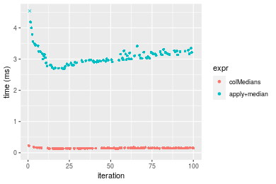
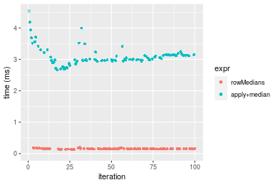Table: Benchmarking of colMedians() and rowMedians() on integer+100x100 data (original and transposed). The top panel shows times in milliseconds and the bottom panel shows relative times.

	expr	min	lq	mean	median	uq	max
1	colMedians	127.340	140.5820	147.0973	144.952	150.4695	229.001
2	rowMedians	132.543	146.7965	152.8494	151.171	155.4980	200.015

	expr	min	lq	mean	median	uq	max
1	colMedians	1.000000	1.000000	1.000000	1.000000	1.000000	1.0000000
2	rowMedians	1.040859	1.044205	1.039105	1.042904	1.033419	0.8734241

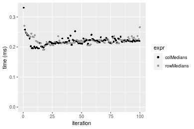
Figure: Benchmarking of colMedians() and rowMedians() on integer+100x100 data (original and transposed). Outliers are displayed as crosses. Times are in milliseconds.

1000x10 integer matrix

> X <- data[["1000x10"]]
> gc()
          used  (Mb) gc trigger  (Mb) max used  (Mb)
Ncells 5242187 280.0    8529671 455.6  8529671 455.6
Vcells 9791069  74.7   31876688 243.2 60562128 462.1
> colStats <- microbenchmark(colMedians = colMedians(X, na.rm = FALSE), `apply+median` = apply(X, MARGIN = 2L, 
+     FUN = median, na.rm = FALSE), unit = "ms")
> X <- t(X)
> gc()
          used  (Mb) gc trigger  (Mb) max used  (Mb)
Ncells 5242163 280.0    8529671 455.6  8529671 455.6
Vcells 9796082  74.8   31876688 243.2 60562128 462.1
> rowStats <- microbenchmark(rowMedians = rowMedians(X, na.rm = FALSE), `apply+median` = apply(X, MARGIN = 1L, 
+     FUN = median, na.rm = FALSE), unit = "ms")

Table: Benchmarking of colMedians() and apply+median() on integer+1000x10 data. The top panel shows times in milliseconds and the bottom panel shows relative times.

	expr	min	lq	mean	median	uq	max
1	colMedians	0.113615	0.118650	0.1391206	0.1365785	0.1496255	0.210331
2	apply+median	0.467260	0.495739	0.5718556	0.5475755	0.6248200	0.918998

	expr	min	lq	mean	median	uq	max
1	colMedians	1.000000	1.000000	1.000000	1.000000	1.000000	1.000000
2	apply+median	4.112661	4.178163	4.110501	4.009236	4.175892	4.369294

Table: Benchmarking of rowMedians() and apply+median() on integer+1000x10 data (transposed). The top panel shows times in milliseconds and the bottom panel shows relative times.

	expr	min	lq	mean	median	uq	max
1	rowMedians	0.116880	0.1204105	0.1424556	0.1341970	0.1559945	0.214430
2	apply+median	0.466145	0.4931330	0.5716402	0.5507485	0.6267335	0.918222

	expr	min	lq	mean	median	uq	max
1	rowMedians	1.000000	1.000000	1.00000	1.00000	1.000000	1.000000
2	apply+median	3.988236	4.095432	4.01276	4.10403	4.017664	4.282153

Figure: Benchmarking of colMedians() and apply+median() on integer+1000x10 data as well as rowMedians() and apply+median() on the same data transposed. Outliers are displayed as crosses. Times are in milliseconds.

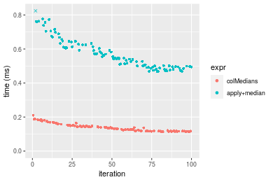
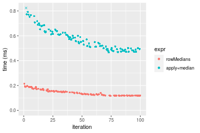Table: Benchmarking of colMedians() and rowMedians() on integer+1000x10 data (original and transposed). The top panel shows times in milliseconds and the bottom panel shows relative times.

	expr	min	lq	mean	median	uq	max
2	rowMedians	116.880	120.4105	142.4556	134.1970	155.9945	214.430
1	colMedians	113.615	118.6500	139.1207	136.5785	149.6255	210.331

	expr	min	lq	mean	median	uq	max
2	rowMedians	1.0000000	1.0000000	1.0000000	1.000000	1.0000000	1.0000000
1	colMedians	0.9720654	0.9853792	0.9765894	1.017746	0.9591716	0.9808842

Figure: Benchmarking of colMedians() and rowMedians() on integer+1000x10 data (original and transposed). Outliers are displayed as crosses. Times are in milliseconds.

10x1000 integer matrix

> X <- data[["10x1000"]]
> gc()
          used  (Mb) gc trigger  (Mb) max used  (Mb)
Ncells 5242375 280.0    8529671 455.6  8529671 455.6
Vcells 9791749  74.8   31876688 243.2 60562128 462.1
> colStats <- microbenchmark(colMedians = colMedians(X, na.rm = FALSE), `apply+median` = apply(X, MARGIN = 2L, 
+     FUN = median, na.rm = FALSE), unit = "ms")
> X <- t(X)
> gc()
          used  (Mb) gc trigger  (Mb) max used  (Mb)
Ncells 5242351 280.0    8529671 455.6  8529671 455.6
Vcells 9796762  74.8   31876688 243.2 60562128 462.1
> rowStats <- microbenchmark(rowMedians = rowMedians(X, na.rm = FALSE), `apply+median` = apply(X, MARGIN = 1L, 
+     FUN = median, na.rm = FALSE), unit = "ms")

Table: Benchmarking of colMedians() and apply+median() on integer+10x1000 data. The top panel shows times in milliseconds and the bottom panel shows relative times.

	expr	min	lq	mean	median	uq	max
1	colMedians	0.144102	0.157876	0.1714867	0.1723645	0.1819535	0.217141
2	apply+median	24.215789	27.295327	28.3589666	27.6258305	28.2971200	49.793969

	expr	min	lq	mean	median	uq	max
1	colMedians	1.0000	1.0000	1.0000	1.0000	1.0000	1.0000
2	apply+median	168.0462	172.8909	165.3713	160.2756	155.5184	229.3163

Table: Benchmarking of rowMedians() and apply+median() on integer+10x1000 data (transposed). The top panel shows times in milliseconds and the bottom panel shows relative times.

	expr	min	lq	mean	median	uq	max
1	rowMedians	0.147904	0.1637175	0.1773978	0.182425	0.188922	0.289775
2	apply+median	25.153866	27.6570375	28.4921616	28.154947	28.639067	34.371020

	expr	min	lq	mean	median	uq	max
1	rowMedians	1.0000	1.0000	1.0000	1.0000	1.000	1.0000
2	apply+median	170.0689	168.9315	160.6117	154.3371	151.592	118.6128

Figure: Benchmarking of colMedians() and apply+median() on integer+10x1000 data as well as rowMedians() and apply+median() on the same data transposed. Outliers are displayed as crosses. Times are in milliseconds.

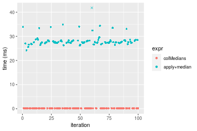
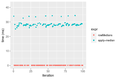Table: Benchmarking of colMedians() and rowMedians() on integer+10x1000 data (original and transposed). The top panel shows times in milliseconds and the bottom panel shows relative times.

	expr	min	lq	mean	median	uq	max
1	colMedians	144.102	157.8760	171.4867	172.3645	181.9535	217.141
2	rowMedians	147.904	163.7175	177.3979	182.4250	188.9220	289.775

	expr	min	lq	mean	median	uq	max
1	colMedians	1.000000	1.000000	1.00000	1.000000	1.000000	1.000000
2	rowMedians	1.026384	1.037001	1.03447	1.058368	1.038298	1.334502

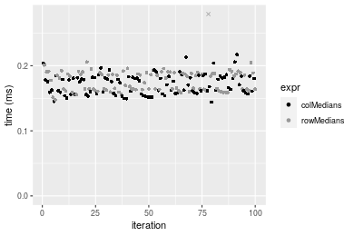
Figure: Benchmarking of colMedians() and rowMedians() on integer+10x1000 data (original and transposed). Outliers are displayed as crosses. Times are in milliseconds.

100x1000 integer matrix

> X <- data[["100x1000"]]
> gc()
          used  (Mb) gc trigger  (Mb) max used  (Mb)
Ncells 5242556 280.0    8529671 455.6  8529671 455.6
Vcells 9792224  74.8   31876688 243.2 60562128 462.1
> colStats <- microbenchmark(colMedians = colMedians(X, na.rm = FALSE), `apply+median` = apply(X, MARGIN = 2L, 
+     FUN = median, na.rm = FALSE), unit = "ms")
> X <- t(X)
> gc()
          used  (Mb) gc trigger  (Mb) max used  (Mb)
Ncells 5242532 280.0    8529671 455.6  8529671 455.6
Vcells 9842237  75.1   31876688 243.2 60562128 462.1
> rowStats <- microbenchmark(rowMedians = rowMedians(X, na.rm = FALSE), `apply+median` = apply(X, MARGIN = 1L, 
+     FUN = median, na.rm = FALSE), unit = "ms")

Table: Benchmarking of colMedians() and apply+median() on integer+100x1000 data. The top panel shows times in milliseconds and the bottom panel shows relative times.

	expr	min	lq	mean	median	uq	max
1	colMedians	1.374103	1.451085	1.480879	1.472018	1.493628	1.765821
2	apply+median	27.910714	30.666674	31.738819	31.045874	31.455668	42.046024

	expr	min	lq	mean	median	uq	max
1	colMedians	1.00000	1.00000	1.00000	1.00000	1.00000	1.00000
2	apply+median	20.31195	21.13362	21.43242	21.09069	21.05991	23.81103

Table: Benchmarking of rowMedians() and apply+median() on integer+100x1000 data (transposed). The top panel shows times in milliseconds and the bottom panel shows relative times.

	expr	min	lq	mean	median	uq	max
1	rowMedians	1.404421	1.496287	1.558611	1.556288	1.610146	1.698434
2	apply+median	27.623059	30.747152	31.927814	31.235588	31.795802	42.329560

	expr	min	lq	mean	median	uq	max
1	rowMedians	1.00000	1.00000	1.00000	1.00000	1.00000	1.0000
2	apply+median	19.66865	20.54897	20.48479	20.07057	19.74715	24.9227

Figure: Benchmarking of colMedians() and apply+median() on integer+100x1000 data as well as rowMedians() and apply+median() on the same data transposed. Outliers are displayed as crosses. Times are in milliseconds.

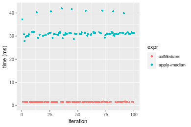
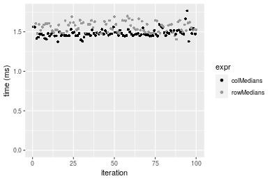
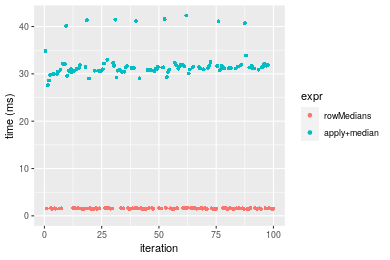Table: Benchmarking of colMedians() and rowMedians() on integer+100x1000 data (original and transposed). The top panel shows times in milliseconds and the bottom panel shows relative times.

	expr	min	lq	mean	median	uq	max
1	colMedians	1.374103	1.451085	1.480879	1.472018	1.493628	1.765821
2	rowMedians	1.404421	1.496287	1.558611	1.556288	1.610146	1.698434

	expr	min	lq	mean	median	uq	max
1	colMedians	1.000000	1.000000	1.00000	1.000000	1.000000	1.0000000
2	rowMedians	1.022064	1.031151	1.05249	1.057248	1.078011	0.9618381

Figure: Benchmarking of colMedians() and rowMedians() on integer+100x1000 data (original and transposed). Outliers are displayed as crosses. Times are in milliseconds.

1000x100 integer matrix

> X <- data[["1000x100"]]
> gc()
          used  (Mb) gc trigger  (Mb) max used  (Mb)
Ncells 5242752 280.0    8529671 455.6  8529671 455.6
Vcells 9792813  74.8   31876688 243.2 60562128 462.1
> colStats <- microbenchmark(colMedians = colMedians(X, na.rm = FALSE), `apply+median` = apply(X, MARGIN = 2L, 
+     FUN = median, na.rm = FALSE), unit = "ms")
> X <- t(X)
> gc()
          used  (Mb) gc trigger  (Mb) max used  (Mb)
Ncells 5242728 280.0    8529671 455.6  8529671 455.6
Vcells 9842826  75.1   31876688 243.2 60562128 462.1
> rowStats <- microbenchmark(rowMedians = rowMedians(X, na.rm = FALSE), `apply+median` = apply(X, MARGIN = 1L, 
+     FUN = median, na.rm = FALSE), unit = "ms")

Table: Benchmarking of colMedians() and apply+median() on integer+1000x100 data. The top panel shows times in milliseconds and the bottom panel shows relative times.

	expr	min	lq	mean	median	uq	max
1	colMedians	1.117822	1.276309	1.291809	1.284461	1.313016	1.851671
2	apply+median	4.466651	5.017188	5.249548	5.090154	5.221628	15.406186

	expr	min	lq	mean	median	uq	max
1	colMedians	1.000000	1.000000	1.000000	1.000000	1.00000	1.000000
2	apply+median	3.995852	3.931014	4.063718	3.962872	3.97682	8.320153

Table: Benchmarking of rowMedians() and apply+median() on integer+1000x100 data (transposed). The top panel shows times in milliseconds and the bottom panel shows relative times.

	expr	min	lq	mean	median	uq	max
1	rowMedians	1.144068	1.302847	1.313454	1.313314	1.324774	1.574031
2	apply+median	4.438241	4.986463	5.178526	5.039875	5.089077	15.821266

	expr	min	lq	mean	median	uq	max
1	rowMedians	1.000000	1.00000	1.000000	1.000000	1.000000	1.00000
2	apply+median	3.879351	3.82736	3.942678	3.837526	3.841467	10.05143

Figure: Benchmarking of colMedians() and apply+median() on integer+1000x100 data as well as rowMedians() and apply+median() on the same data transposed. Outliers are displayed as crosses. Times are in milliseconds.

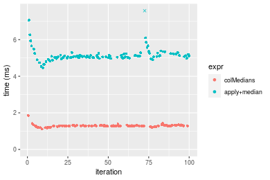
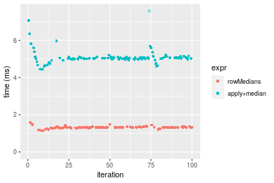Table: Benchmarking of colMedians() and rowMedians() on integer+1000x100 data (original and transposed). The top panel shows times in milliseconds and the bottom panel shows relative times.

	expr	min	lq	mean	median	uq	max
1	colMedians	1.117822	1.276309	1.291809	1.284461	1.313016	1.851671
2	rowMedians	1.144068	1.302847	1.313454	1.313314	1.324774	1.574031

	expr	min	lq	mean	median	uq	max
1	colMedians	1.00000	1.000000	1.000000	1.000000	1.000000	1.0000000
2	rowMedians	1.02348	1.020792	1.016755	1.022463	1.008955	0.8500598

Figure: Benchmarking of colMedians() and rowMedians() on integer+1000x100 data (original and transposed). Outliers are displayed as crosses. Times are in milliseconds.

Data type “double”

Data

> rmatrix <- function(nrow, ncol, mode = c("logical", "double", "integer", "index"), range = c(-100, 
+     +100), na_prob = 0) {
+     mode <- match.arg(mode)
+     n <- nrow * ncol
+     if (mode == "logical") {
+         x <- sample(c(FALSE, TRUE), size = n, replace = TRUE)
+     }     else if (mode == "index") {
+         x <- seq_len(n)
+         mode <- "integer"
+     }     else {
+         x <- runif(n, min = range[1], max = range[2])
+     }
+     storage.mode(x) <- mode
+     if (na_prob > 0) 
+         x[sample(n, size = na_prob * n)] <- NA
+     dim(x) <- c(nrow, ncol)
+     x
+ }
> rmatrices <- function(scale = 10, seed = 1, ...) {
+     set.seed(seed)
+     data <- list()
+     data[[1]] <- rmatrix(nrow = scale * 1, ncol = scale * 1, ...)
+     data[[2]] <- rmatrix(nrow = scale * 10, ncol = scale * 10, ...)
+     data[[3]] <- rmatrix(nrow = scale * 100, ncol = scale * 1, ...)
+     data[[4]] <- t(data[[3]])
+     data[[5]] <- rmatrix(nrow = scale * 10, ncol = scale * 100, ...)
+     data[[6]] <- t(data[[5]])
+     names(data) <- sapply(data, FUN = function(x) paste(dim(x), collapse = "x"))
+     data
+ }
> data <- rmatrices(mode = mode)

Results

10x10 double matrix

> X <- data[["10x10"]]
> gc()
          used  (Mb) gc trigger  (Mb) max used  (Mb)
Ncells 5242934 280.1    8529671 455.6  8529671 455.6
Vcells 9909186  75.7   31876688 243.2 60562128 462.1
> colStats <- microbenchmark(colMedians = colMedians(X, na.rm = FALSE), `apply+median` = apply(X, MARGIN = 2L, 
+     FUN = median, na.rm = FALSE), unit = "ms")
> X <- t(X)
> gc()
          used  (Mb) gc trigger  (Mb) max used  (Mb)
Ncells 5242919 280.1    8529671 455.6  8529671 455.6
Vcells 9909314  75.7   31876688 243.2 60562128 462.1
> rowStats <- microbenchmark(rowMedians = rowMedians(X, na.rm = FALSE), `apply+median` = apply(X, MARGIN = 1L, 
+     FUN = median, na.rm = FALSE), unit = "ms")

Table: Benchmarking of colMedians() and apply+median() on double+10x10 data. The top panel shows times in milliseconds and the bottom panel shows relative times.

	expr	min	lq	mean	median	uq	max
1	colMedians	0.002722	0.003405	0.0048599	0.004527	0.0055105	0.020931
2	apply+median	0.318562	0.330678	0.3679373	0.352705	0.3870845	0.601393

	expr	min	lq	mean	median	uq	max
1	colMedians	1.0000	1.00000	1.00000	1.00000	1.0000	1.00000
2	apply+median	117.0323	97.11542	75.70928	77.91142	70.2449	28.73217

Table: Benchmarking of rowMedians() and apply+median() on double+10x10 data (transposed). The top panel shows times in milliseconds and the bottom panel shows relative times.

	expr	min	lq	mean	median	uq	max
1	rowMedians	0.002799	0.0036850	0.0051966	0.0051590	0.005987	0.017993
2	apply+median	0.304087	0.3250145	0.3618629	0.3496705	0.405575	0.585888

	expr	min	lq	mean	median	uq	max
1	rowMedians	1.0000	1.00000	1.00000	1.00000	1.00000	1.000
2	apply+median	108.6413	88.19932	69.63441	67.77874	67.74261	32.562

Figure: Benchmarking of colMedians() and apply+median() on double+10x10 data as well as rowMedians() and apply+median() on the same data transposed. Outliers are displayed as crosses. Times are in milliseconds.

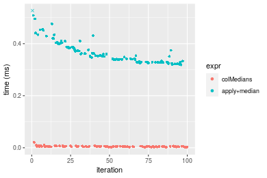
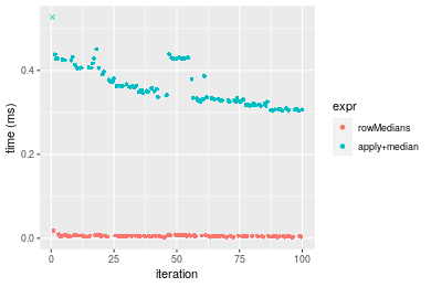Table: Benchmarking of colMedians() and rowMedians() on double+10x10 data (original and transposed). The top panel shows times in milliseconds and the bottom panel shows relative times.

	expr	min	lq	mean	median	uq	max
1	colMedians	2.722	3.405	4.85987	4.527	5.5105	20.931
2	rowMedians	2.799	3.685	5.19661	5.159	5.9870	17.993

	expr	min	lq	mean	median	uq	max
1	colMedians	1.000000	1.000000	1.00000	1.000000	1.000000	1.000000
2	rowMedians	1.028288	1.082232	1.06929	1.139607	1.086471	0.859634

Figure: Benchmarking of colMedians() and rowMedians() on double+10x10 data (original and transposed). Outliers are displayed as crosses. Times are in milliseconds.

100x100 double matrix

> X <- data[["100x100"]]
> gc()
          used  (Mb) gc trigger  (Mb) max used  (Mb)
Ncells 5243130 280.1    8529671 455.6  8529671 455.6
Vcells 9909326  75.7   31876688 243.2 60562128 462.1
> colStats <- microbenchmark(colMedians = colMedians(X, na.rm = FALSE), `apply+median` = apply(X, MARGIN = 2L, 
+     FUN = median, na.rm = FALSE), unit = "ms")
> X <- t(X)
> gc()
          used  (Mb) gc trigger  (Mb) max used  (Mb)
Ncells 5243106 280.1    8529671 455.6  8529671 455.6
Vcells 9919339  75.7   31876688 243.2 60562128 462.1
> rowStats <- microbenchmark(rowMedians = rowMedians(X, na.rm = FALSE), `apply+median` = apply(X, MARGIN = 1L, 
+     FUN = median, na.rm = FALSE), unit = "ms")

Table: Benchmarking of colMedians() and apply+median() on double+100x100 data. The top panel shows times in milliseconds and the bottom panel shows relative times.

	expr	min	lq	mean	median	uq	max
1	colMedians	0.195424	0.212914	0.2197392	0.218946	0.223244	0.330914
2	apply+median	2.764987	3.066848	3.1859469	3.141621	3.293928	4.702083

	expr	min	lq	mean	median	uq	max
1	colMedians	1.00000	1.00000	1.00000	1.00000	1.00000	1.00000
2	apply+median	14.14866	14.40417	14.49877	14.34884	14.75484	14.20938

Table: Benchmarking of rowMedians() and apply+median() on double+100x100 data (transposed). The top panel shows times in milliseconds and the bottom panel shows relative times.

	expr	min	lq	mean	median	uq	max
1	rowMedians	0.190917	0.2133255	0.2207082	0.21938	0.225468	0.270784
2	apply+median	2.752276	3.0632630	3.2004389	3.14504	3.330661	4.719369

	expr	min	lq	mean	median	uq	max
1	rowMedians	1.00000	1.00000	1.00000	1.00000	1.00000	1.00000
2	apply+median	14.41609	14.35957	14.50077	14.33604	14.77221	17.42854

Figure: Benchmarking of colMedians() and apply+median() on double+100x100 data as well as rowMedians() and apply+median() on the same data transposed. Outliers are displayed as crosses. Times are in milliseconds.

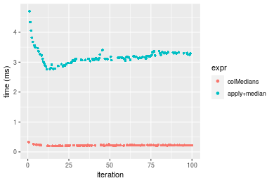
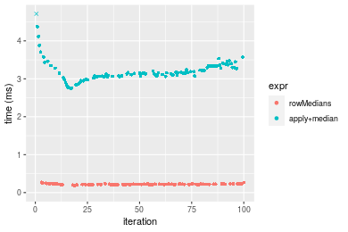Table: Benchmarking of colMedians() and rowMedians() on double+100x100 data (original and transposed). The top panel shows times in milliseconds and the bottom panel shows relative times.

	expr	min	lq	mean	median	uq	max
1	colMedians	195.424	212.9140	219.7392	218.946	223.244	330.914
2	rowMedians	190.917	213.3255	220.7081	219.380	225.468	270.784

	expr	min	lq	mean	median	uq	max
1	colMedians	1.0000000	1.000000	1.00000	1.000000	1.000000	1.0000000
2	rowMedians	0.9769373	1.001933	1.00441	1.001982	1.009962	0.8182912

Figure: Benchmarking of colMedians() and rowMedians() on double+100x100 data (original and transposed). Outliers are displayed as crosses. Times are in milliseconds.

1000x10 double matrix

> X <- data[["1000x10"]]
> gc()
          used  (Mb) gc trigger  (Mb) max used  (Mb)
Ncells 5243315 280.1    8529671 455.6  8529671 455.6
Vcells 9910207  75.7   31876688 243.2 60562128 462.1
> colStats <- microbenchmark(colMedians = colMedians(X, na.rm = FALSE), `apply+median` = apply(X, MARGIN = 2L, 
+     FUN = median, na.rm = FALSE), unit = "ms")
> X <- t(X)
> gc()
          used  (Mb) gc trigger  (Mb) max used  (Mb)
Ncells 5243297 280.1    8529671 455.6  8529671 455.6
Vcells 9920230  75.7   31876688 243.2 60562128 462.1
> rowStats <- microbenchmark(rowMedians = rowMedians(X, na.rm = FALSE), `apply+median` = apply(X, MARGIN = 1L, 
+     FUN = median, na.rm = FALSE), unit = "ms")

Table: Benchmarking of colMedians() and apply+median() on double+1000x10 data. The top panel shows times in milliseconds and the bottom panel shows relative times.

	expr	min	lq	mean	median	uq	max
1	colMedians	0.175335	0.1829445	0.2131880	0.198377	0.229199	0.308704
2	apply+median	0.531410	0.5498355	0.6345319	0.585643	0.688513	1.033381

	expr	min	lq	mean	median	uq	max
1	colMedians	1.000000	1.000000	1.000000	1.000000	1.000000	1.000000
2	apply+median	3.030827	3.005477	2.976396	2.952172	3.003996	3.347482

Table: Benchmarking of rowMedians() and apply+median() on double+1000x10 data (transposed). The top panel shows times in milliseconds and the bottom panel shows relative times.

	expr	min	lq	mean	median	uq	max
1	rowMedians	0.176283	0.1859945	0.2198387	0.2039295	0.2355145	0.389123
2	apply+median	0.526611	0.5679495	0.6610664	0.6418115	0.7123670	1.326834

	expr	min	lq	mean	median	uq	max
1	rowMedians	1.000000	1.000000	1.000000	1.000000	1.000000	1.000000
2	apply+median	2.987305	3.053582	3.007052	3.147222	3.024727	3.409806

Figure: Benchmarking of colMedians() and apply+median() on double+1000x10 data as well as rowMedians() and apply+median() on the same data transposed. Outliers are displayed as crosses. Times are in milliseconds.

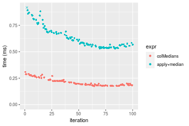
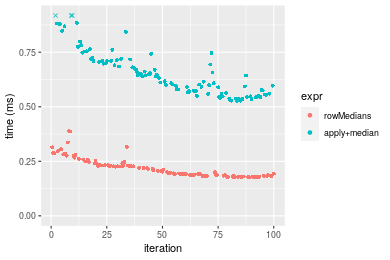Table: Benchmarking of colMedians() and rowMedians() on double+1000x10 data (original and transposed). The top panel shows times in milliseconds and the bottom panel shows relative times.

	expr	min	lq	mean	median	uq	max
1	colMedians	175.335	182.9445	213.1880	198.3770	229.1990	308.704
2	rowMedians	176.283	185.9945	219.8387	203.9295	235.5145	389.123

	expr	min	lq	mean	median	uq	max
1	colMedians	1.000000	1.000000	1.000000	1.00000	1.000000	1.000000
2	rowMedians	1.005407	1.016672	1.031197	1.02799	1.027555	1.260505

Figure: Benchmarking of colMedians() and rowMedians() on double+1000x10 data (original and transposed). Outliers are displayed as crosses. Times are in milliseconds.

10x1000 double matrix

> X <- data[["10x1000"]]
> gc()
          used  (Mb) gc trigger  (Mb) max used  (Mb)
Ncells 5243509 280.1    8529671 455.6  8529671 455.6
Vcells 9911262  75.7   31876688 243.2 60562128 462.1
> colStats <- microbenchmark(colMedians = colMedians(X, na.rm = FALSE), `apply+median` = apply(X, MARGIN = 2L, 
+     FUN = median, na.rm = FALSE), unit = "ms")
> X <- t(X)
> gc()
          used  (Mb) gc trigger  (Mb) max used  (Mb)
Ncells 5243485 280.1    8529671 455.6  8529671 455.6
Vcells 9921275  75.7   31876688 243.2 60562128 462.1
> rowStats <- microbenchmark(rowMedians = rowMedians(X, na.rm = FALSE), `apply+median` = apply(X, MARGIN = 1L, 
+     FUN = median, na.rm = FALSE), unit = "ms")

Table: Benchmarking of colMedians() and apply+median() on double+10x1000 data. The top panel shows times in milliseconds and the bottom panel shows relative times.

	expr	min	lq	mean	median	uq	max
1	colMedians	0.205459	0.2310795	0.2412473	0.243109	0.249687	0.272166
2	apply+median	24.932106	28.1365430	28.9532241	28.356629	29.045983	35.188701

	expr	min	lq	mean	median	uq	max
1	colMedians	1.0000	1.0000	1.0000	1.0000	1.0000	1.0000
2	apply+median	121.3483	121.7613	120.0147	116.6416	116.3296	129.2913

Table: Benchmarking of rowMedians() and apply+median() on double+10x1000 data (transposed). The top panel shows times in milliseconds and the bottom panel shows relative times.

	expr	min	lq	mean	median	uq	max
1	rowMedians	0.217118	0.231363	0.2432768	0.244235	0.250688	0.306857
2	apply+median	25.173491	28.197331	29.1656326	28.556639	29.053978	49.903651

	expr	min	lq	mean	median	uq	max
1	rowMedians	1.0000	1.0000	1.0000	1.0000	1.000	1.0000
2	apply+median	115.9438	121.8749	119.8866	116.9228	115.897	162.6284

Figure: Benchmarking of colMedians() and apply+median() on double+10x1000 data as well as rowMedians() and apply+median() on the same data transposed. Outliers are displayed as crosses. Times are in milliseconds.

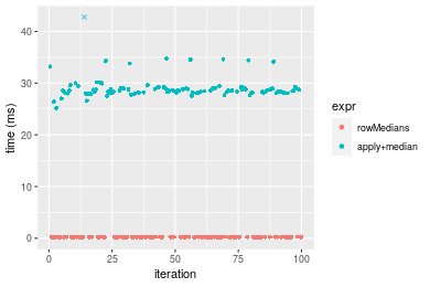Table: Benchmarking of colMedians() and rowMedians() on double+10x1000 data (original and transposed). The top panel shows times in milliseconds and the bottom panel shows relative times.

	expr	min	lq	mean	median	uq	max
1	colMedians	205.459	231.0795	241.2473	243.109	249.687	272.166
2	rowMedians	217.118	231.3630	243.2768	244.235	250.688	306.857

	expr	min	lq	mean	median	uq	max
1	colMedians	1.000000	1.000000	1.000000	1.000000	1.000000	1.000000
2	rowMedians	1.056746	1.001227	1.008412	1.004632	1.004009	1.127463

Figure: Benchmarking of colMedians() and rowMedians() on double+10x1000 data (original and transposed). Outliers are displayed as crosses. Times are in milliseconds.

100x1000 double matrix

> X <- data[["100x1000"]]
> gc()
          used  (Mb) gc trigger  (Mb) max used  (Mb)
Ncells 5243690 280.1    8529671 455.6  8529671 455.6
Vcells 9911380  75.7   31876688 243.2 60562128 462.1
> colStats <- microbenchmark(colMedians = colMedians(X, na.rm = FALSE), `apply+median` = apply(X, MARGIN = 2L, 
+     FUN = median, na.rm = FALSE), unit = "ms")
> X <- t(X)
> gc()
           used  (Mb) gc trigger  (Mb) max used  (Mb)
Ncells  5243666 280.1    8529671 455.6  8529671 455.6
Vcells 10011393  76.4   31876688 243.2 60562128 462.1
> rowStats <- microbenchmark(rowMedians = rowMedians(X, na.rm = FALSE), `apply+median` = apply(X, MARGIN = 1L, 
+     FUN = median, na.rm = FALSE), unit = "ms")

Table: Benchmarking of colMedians() and apply+median() on double+100x1000 data. The top panel shows times in milliseconds and the bottom panel shows relative times.

	expr	min	lq	mean	median	uq	max
1	colMedians	1.991339	2.163176	2.212279	2.201229	2.239289	3.22232
2	apply+median	28.649616	31.665022	33.011730	32.111881	32.701452	45.12525

	expr	min	lq	mean	median	uq	max
1	colMedians	1.00000	1.00000	1.00000	1.00000	1.0000	1.00000
2	apply+median	14.38711	14.63821	14.92205	14.58816	14.6035	14.00396

Table: Benchmarking of rowMedians() and apply+median() on double+100x1000 data (transposed). The top panel shows times in milliseconds and the bottom panel shows relative times.

	expr	min	lq	mean	median	uq	max
1	rowMedians	1.986987	2.208758	2.288274	2.297048	2.341113	3.016235
2	apply+median	29.213197	31.805172	36.488748	32.142513	32.771625	390.646579

	expr	min	lq	mean	median	uq	max
1	rowMedians	1.00000	1.00000	1.00000	1.00000	1.00000	1.0000
2	apply+median	14.70226	14.39957	15.94597	13.99297	13.99831	129.5146

Figure: Benchmarking of colMedians() and apply+median() on double+100x1000 data as well as rowMedians() and apply+median() on the same data transposed. Outliers are displayed as crosses. Times are in milliseconds.

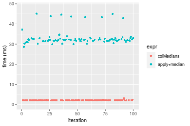
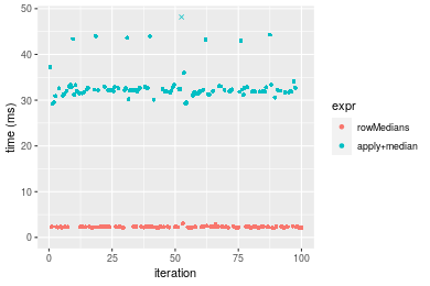Table: Benchmarking of colMedians() and rowMedians() on double+100x1000 data (original and transposed). The top panel shows times in milliseconds and the bottom panel shows relative times.

	expr	min	lq	mean	median	uq	max
1	colMedians	1.991339	2.163176	2.212279	2.201229	2.239289	3.222320
2	rowMedians	1.986987	2.208758	2.288274	2.297048	2.341113	3.016235

	expr	min	lq	mean	median	uq	max
1	colMedians	1.0000000	1.000000	1.000000	1.000000	1.000000	1.0000000
2	rowMedians	0.9978145	1.021072	1.034352	1.043529	1.045472	0.9360445

Figure: Benchmarking of colMedians() and rowMedians() on double+100x1000 data (original and transposed). Outliers are displayed as crosses. Times are in milliseconds.

1000x100 double matrix

> X <- data[["1000x100"]]
> gc()
          used  (Mb) gc trigger  (Mb) max used  (Mb)
Ncells 5243886 280.1    8529671 455.6  8529671 455.6
Vcells 9912619  75.7   31876688 243.2 60562128 462.1
> colStats <- microbenchmark(colMedians = colMedians(X, na.rm = FALSE), `apply+median` = apply(X, MARGIN = 2L, 
+     FUN = median, na.rm = FALSE), unit = "ms")
> X <- t(X)
> gc()
           used  (Mb) gc trigger  (Mb) max used  (Mb)
Ncells  5243862 280.1    8529671 455.6  8529671 455.6
Vcells 10012632  76.4   31876688 243.2 60562128 462.1
> rowStats <- microbenchmark(rowMedians = rowMedians(X, na.rm = FALSE), `apply+median` = apply(X, MARGIN = 1L, 
+     FUN = median, na.rm = FALSE), unit = "ms")

Table: Benchmarking of colMedians() and apply+median() on double+1000x100 data. The top panel shows times in milliseconds and the bottom panel shows relative times.

	expr	min	lq	mean	median	uq	max
1	colMedians	1.758738	2.000690	2.029535	2.024788	2.062974	2.853849
2	apply+median	5.150175	5.782103	6.113051	5.866638	5.971119	14.670965

	expr	min	lq	mean	median	uq	max
1	colMedians	1.000000	1.000000	1.000000	1.000000	1.000000	1.000000
2	apply+median	2.928336	2.890054	3.012045	2.897409	2.894423	5.140764

Table: Benchmarking of rowMedians() and apply+median() on double+1000x100 data (transposed). The top panel shows times in milliseconds and the bottom panel shows relative times.

	expr	min	lq	mean	median	uq	max
1	rowMedians	1.749699	1.991984	2.039428	2.032979	2.076482	2.413104
2	apply+median	5.179044	5.814283	6.093613	5.871463	6.005294	15.101126

	expr	min	lq	mean	median	uq	max
1	rowMedians	1.000000	1.00000	1.000000	1.000000	1.000000	1.000000
2	apply+median	2.959963	2.91884	2.987903	2.888108	2.892052	6.257967

Figure: Benchmarking of colMedians() and apply+median() on double+1000x100 data as well as rowMedians() and apply+median() on the same data transposed. Outliers are displayed as crosses. Times are in milliseconds.

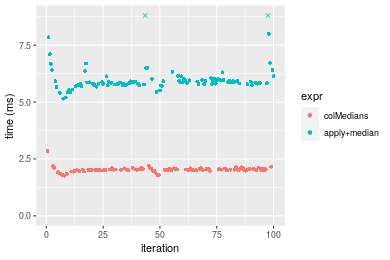
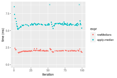Table: Benchmarking of colMedians() and rowMedians() on double+1000x100 data (original and transposed). The top panel shows times in milliseconds and the bottom panel shows relative times.

	expr	min	lq	mean	median	uq	max
1	colMedians	1.758738	2.000690	2.029535	2.024788	2.062974	2.853849
2	rowMedians	1.749699	1.991984	2.039428	2.032979	2.076482	2.413104

	expr	min	lq	mean	median	uq	max
1	colMedians	1.0000000	1.0000000	1.000000	1.000000	1.000000	1.0000000
2	rowMedians	0.9948605	0.9956485	1.004875	1.004045	1.006548	0.8455612

Figure: Benchmarking of colMedians() and rowMedians() on double+1000x100 data (original and transposed). Outliers are displayed as crosses. Times are in milliseconds.

Appendix

Session information

R version 4.1.1 Patched (2021-08-10 r80727)
Platform: x86_64-pc-linux-gnu (64-bit)
Running under: Ubuntu 18.04.5 LTS

Matrix products: default
BLAS:   /home/hb/software/R-devel/R-4-1-branch/lib/R/lib/libRblas.so
LAPACK: /home/hb/software/R-devel/R-4-1-branch/lib/R/lib/libRlapack.so

locale:
 [1] LC_CTYPE=en_US.UTF-8       LC_NUMERIC=C              
 [3] LC_TIME=en_US.UTF-8        LC_COLLATE=en_US.UTF-8    
 [5] LC_MONETARY=en_US.UTF-8    LC_MESSAGES=en_US.UTF-8   
 [7] LC_PAPER=en_US.UTF-8       LC_NAME=C                 
 [9] LC_ADDRESS=C               LC_TELEPHONE=C            
[11] LC_MEASUREMENT=en_US.UTF-8 LC_IDENTIFICATION=C       

attached base packages:
[1] stats     graphics  grDevices utils     datasets  methods   base     

other attached packages:
[1] microbenchmark_1.4-7   matrixStats_0.60.1     ggplot2_3.3.5         
[4] knitr_1.33             R.devices_2.17.0       R.utils_2.10.1        
[7] R.oo_1.24.0            R.methodsS3_1.8.1-9001 history_0.0.1-9000    

loaded via a namespace (and not attached):
 [1] Biobase_2.52.0          httr_1.4.2              splines_4.1.1          
 [4] bit64_4.0.5             network_1.17.1          assertthat_0.2.1       
 [7] highr_0.9               stats4_4.1.1            blob_1.2.2             
[10] GenomeInfoDbData_1.2.6  robustbase_0.93-8       pillar_1.6.2           
[13] RSQLite_2.2.8           lattice_0.20-44         glue_1.4.2             
[16] digest_0.6.27           XVector_0.32.0          colorspace_2.0-2       
[19] Matrix_1.3-4            XML_3.99-0.7            pkgconfig_2.0.3        
[22] zlibbioc_1.38.0         genefilter_1.74.0       purrr_0.3.4            
[25] ergm_4.1.2              xtable_1.8-4            scales_1.1.1           
[28] tibble_3.1.4            annotate_1.70.0         KEGGREST_1.32.0        
[31] farver_2.1.0            generics_0.1.0          IRanges_2.26.0         
[34] ellipsis_0.3.2          cachem_1.0.6            withr_2.4.2            
[37] BiocGenerics_0.38.0     mime_0.11               survival_3.2-13        
[40] magrittr_2.0.1          crayon_1.4.1            statnet.common_4.5.0   
[43] memoise_2.0.0           laeken_0.5.1            fansi_0.5.0            
[46] R.cache_0.15.0          MASS_7.3-54             R.rsp_0.44.0           
[49] progressr_0.8.0         tools_4.1.1             lifecycle_1.0.0        
[52] S4Vectors_0.30.0        trust_0.1-8             munsell_0.5.0          
[55] tabby_0.0.1-9001        AnnotationDbi_1.54.1    Biostrings_2.60.2      
[58] compiler_4.1.1          GenomeInfoDb_1.28.1     rlang_0.4.11           
[61] grid_4.1.1              RCurl_1.98-1.4          cwhmisc_6.6            
[64] rappdirs_0.3.3          startup_0.15.0          labeling_0.4.2         
[67] bitops_1.0-7            base64enc_0.1-3         boot_1.3-28            
[70] gtable_0.3.0            DBI_1.1.1               markdown_1.1           
[73] R6_2.5.1                lpSolveAPI_5.5.2.0-17.7 rle_0.9.2              
[76] dplyr_1.0.7             fastmap_1.1.0           bit_4.0.4              
[79] utf8_1.2.2              parallel_4.1.1          Rcpp_1.0.7             
[82] vctrs_0.3.8             png_0.1-7               DEoptimR_1.0-9         
[85] tidyselect_1.1.1        xfun_0.25               coda_0.19-4            

Total processing time was 52.96 secs.

Reproducibility

To reproduce this report, do:

html <- matrixStats:::benchmark('colMedians')