matrixStats.benchmarks

colCounts() and rowCounts() benchmarks on subsetted computation

This report benchmark the performance of colCounts() and rowCounts() on subsetted computation.

Data type “logical”

Data

> rmatrix <- function(nrow, ncol, mode = c("logical", "double", "integer", "index"), range = c(-100, 
+     +100), na_prob = 0) {
+     mode <- match.arg(mode)
+     n <- nrow * ncol
+     if (mode == "logical") {
+         x <- sample(c(FALSE, TRUE), size = n, replace = TRUE)
+     }     else if (mode == "index") {
+         x <- seq_len(n)
+         mode <- "integer"
+     }     else {
+         x <- runif(n, min = range[1], max = range[2])
+     }
+     storage.mode(x) <- mode
+     if (na_prob > 0) 
+         x[sample(n, size = na_prob * n)] <- NA
+     dim(x) <- c(nrow, ncol)
+     x
+ }
> rmatrices <- function(scale = 10, seed = 1, ...) {
+     set.seed(seed)
+     data <- list()
+     data[[1]] <- rmatrix(nrow = scale * 1, ncol = scale * 1, ...)
+     data[[2]] <- rmatrix(nrow = scale * 10, ncol = scale * 10, ...)
+     data[[3]] <- rmatrix(nrow = scale * 100, ncol = scale * 1, ...)
+     data[[4]] <- t(data[[3]])
+     data[[5]] <- rmatrix(nrow = scale * 10, ncol = scale * 100, ...)
+     data[[6]] <- t(data[[5]])
+     names(data) <- sapply(data, FUN = function(x) paste(dim(x), collapse = "x"))
+     data
+ }
> data <- rmatrices(mode = mode)

Results

10x10 matrix

> X <- data[["10x10"]]
> rows <- sample.int(nrow(X), size = nrow(X) * 0.7)
> cols <- sample.int(ncol(X), size = ncol(X) * 0.7)
> X_S <- X[rows, cols]
> value <- 42

> colStats <- microbenchmark(colCounts_X_S = colCounts(X_S, value = value, na.rm = FALSE), `colCounts(X, rows, cols)` = colCounts(X, 
+     value = value, na.rm = FALSE, rows = rows, cols = cols), `colCounts(X[rows, cols])` = colCounts(X[rows, 
+     cols], value = value, na.rm = FALSE), unit = "ms")

> X <- t(X)
> X_S <- t(X_S)

> rowStats <- microbenchmark(rowCounts_X_S = rowCounts(X_S, value = value, na.rm = FALSE), `rowCounts(X, cols, rows)` = rowCounts(X, 
+     value = value, na.rm = FALSE, rows = cols, cols = rows), `rowCounts(X[cols, rows])` = rowCounts(X[cols, 
+     rows], value = value, na.rm = FALSE), unit = "ms")

Table: Benchmarking of colCounts_X_S(), colCounts(X, rows, cols)() and colCounts(X[rows, cols])() on logical+10x10 data. The top panel shows times in milliseconds and the bottom panel shows relative times.

	expr	min	lq	mean	median	uq	max
1	colCounts_X_S	0.007861	0.0080850	0.0115681	0.008181	0.0082945	0.339868
2	colCounts(X, rows, cols)	0.008249	0.0085180	0.0086985	0.008649	0.0087685	0.012066
3	colCounts(X[rows, cols])	0.009135	0.0095735	0.0098538	0.009728	0.0098950	0.017209

	expr	min	lq	mean	median	uq	max
1	colCounts_X_S	1.000000	1.000000	1.0000000	1.000000	1.000000	1.0000000
2	colCounts(X, rows, cols)	1.049358	1.053556	0.7519428	1.057206	1.057146	0.0355020
3	colCounts(X[rows, cols])	1.162066	1.184106	0.8518080	1.189097	1.192959	0.0506344

Table: Benchmarking of rowCounts_X_S(), rowCounts(X, cols, rows)() and rowCounts(X[cols, rows])() on logical+10x10 data (transposed). The top panel shows times in milliseconds and the bottom panel shows relative times.

	expr	min	lq	mean	median	uq	max
1	rowCounts_X_S	0.006790	0.0070025	0.0072210	0.0071140	0.0072720	0.011651
2	rowCounts(X, cols, rows)	0.007319	0.0074320	0.0106515	0.0075030	0.0076460	0.311765
3	rowCounts(X[cols, rows])	0.007951	0.0082750	0.0084884	0.0083995	0.0085625	0.011150

	expr	min	lq	mean	median	uq	max
1	rowCounts_X_S	1.000000	1.000000	1.000000	1.000000	1.000000	1.0000000
2	rowCounts(X, cols, rows)	1.077909	1.061335	1.475069	1.054681	1.051430	26.7586473
3	rowCounts(X[cols, rows])	1.170987	1.181721	1.175518	1.180700	1.177461	0.9569994

Figure: Benchmarking of colCounts_X_S(), colCounts(X, rows, cols)() and colCounts(X[rows, cols])() on logical+10x10 data as well as rowCounts_X_S(), rowCounts(X, cols, rows)() and rowCounts(X[cols, rows])() on the same data transposed. Outliers are displayed as crosses. Times are in milliseconds.

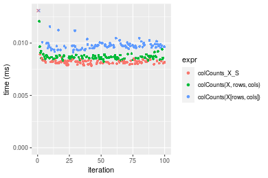
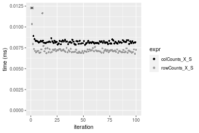
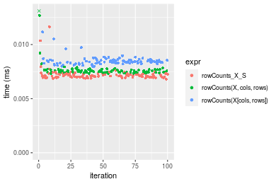Table: Benchmarking of colCounts_X_S() and rowCounts_X_S() on logical+10x10 data (original and transposed). The top panel shows times in milliseconds and the bottom panel shows relative times.

	expr	min	lq	mean	median	uq	max
2	rowCounts_X_S	6.790	7.0025	7.22102	7.114	7.2720	11.651
1	colCounts_X_S	7.861	8.0850	11.56810	8.181	8.2945	339.868

	expr	min	lq	mean	median	uq	max
2	rowCounts_X_S	1.000000	1.000000	1.000000	1.000000	1.000000	1.00000
1	colCounts_X_S	1.157732	1.154588	1.602004	1.149986	1.140608	29.17072

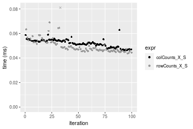
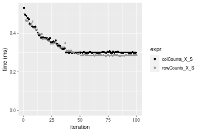
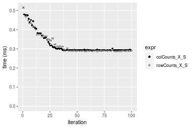
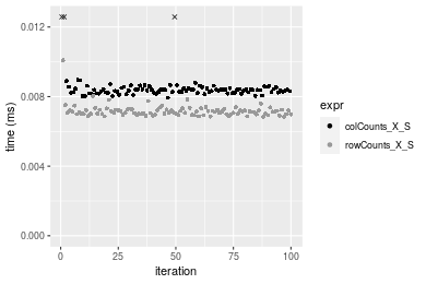
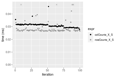
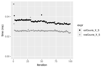
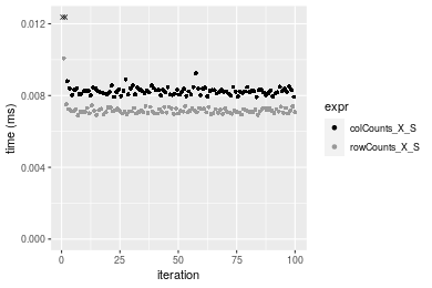
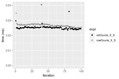
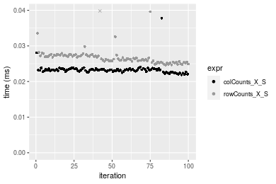
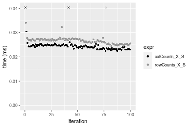
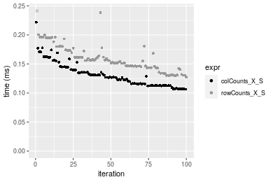
Figure: Benchmarking of colCounts_X_S() and rowCounts_X_S() on logical+10x10 data (original and transposed). Outliers are displayed as crosses. Times are in milliseconds.

100x100 matrix

> X <- data[["100x100"]]
> rows <- sample.int(nrow(X), size = nrow(X) * 0.7)
> cols <- sample.int(ncol(X), size = ncol(X) * 0.7)
> X_S <- X[rows, cols]
> value <- 42

> colStats <- microbenchmark(colCounts_X_S = colCounts(X_S, value = value, na.rm = FALSE), `colCounts(X, rows, cols)` = colCounts(X, 
+     value = value, na.rm = FALSE, rows = rows, cols = cols), `colCounts(X[rows, cols])` = colCounts(X[rows, 
+     cols], value = value, na.rm = FALSE), unit = "ms")

> X <- t(X)
> X_S <- t(X_S)

> rowStats <- microbenchmark(rowCounts_X_S = rowCounts(X_S, value = value, na.rm = FALSE), `rowCounts(X, cols, rows)` = rowCounts(X, 
+     value = value, na.rm = FALSE, rows = cols, cols = rows), `rowCounts(X[cols, rows])` = rowCounts(X[cols, 
+     rows], value = value, na.rm = FALSE), unit = "ms")

Table: Benchmarking of colCounts_X_S(), colCounts(X, rows, cols)() and colCounts(X[rows, cols])() on logical+100x100 data. The top panel shows times in milliseconds and the bottom panel shows relative times.

	expr	min	lq	mean	median	uq	max
2	colCounts(X, rows, cols)	0.046103	0.0498330	0.0553339	0.0535885	0.056785	0.085855
1	colCounts_X_S	0.046855	0.0496065	0.0559248	0.0544480	0.056445	0.087820
3	colCounts(X[rows, cols])	0.061274	0.0651130	0.0717809	0.0704865	0.073310	0.124024

	expr	min	lq	mean	median	uq	max
2	colCounts(X, rows, cols)	1.000000	1.0000000	1.000000	1.000000	1.0000000	1.000000
1	colCounts_X_S	1.016311	0.9954548	1.010679	1.016039	0.9940125	1.022887
3	colCounts(X[rows, cols])	1.329068	1.3066241	1.297232	1.315329	1.2910099	1.444575

Table: Benchmarking of rowCounts_X_S(), rowCounts(X, cols, rows)() and rowCounts(X[cols, rows])() on logical+100x100 data (transposed). The top panel shows times in milliseconds and the bottom panel shows relative times.

	expr	min	lq	mean	median	uq	max
1	rowCounts_X_S	0.042031	0.0453435	0.0486862	0.0492505	0.051206	0.062865
2	rowCounts(X, cols, rows)	0.047862	0.0507645	0.0543945	0.0538780	0.056810	0.101751
3	rowCounts(X[cols, rows])	0.055873	0.0609775	0.0647972	0.0643790	0.068220	0.083495

	expr	min	lq	mean	median	uq	max
1	rowCounts_X_S	1.000000	1.000000	1.000000	1.000000	1.000000	1.000000
2	rowCounts(X, cols, rows)	1.138731	1.119554	1.117246	1.093958	1.109440	1.618564
3	rowCounts(X[cols, rows])	1.329328	1.344790	1.330914	1.307174	1.332266	1.328164

Figure: Benchmarking of colCounts_X_S(), colCounts(X, rows, cols)() and colCounts(X[rows, cols])() on logical+100x100 data as well as rowCounts_X_S(), rowCounts(X, cols, rows)() and rowCounts(X[cols, rows])() on the same data transposed. Outliers are displayed as crosses. Times are in milliseconds.

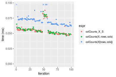
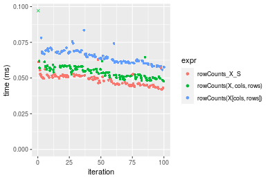Table: Benchmarking of colCounts_X_S() and rowCounts_X_S() on logical+100x100 data (original and transposed). The top panel shows times in milliseconds and the bottom panel shows relative times.

	expr	min	lq	mean	median	uq	max
2	rowCounts_X_S	42.031	45.3435	48.68624	49.2505	51.206	62.865
1	colCounts_X_S	46.855	49.6065	55.92485	54.4480	56.445	87.820

	expr	min	lq	mean	median	uq	max
2	rowCounts_X_S	1.000000	1.000000	1.000000	1.000000	1.000000	1.000000
1	colCounts_X_S	1.114772	1.094016	1.148679	1.105532	1.102312	1.396962

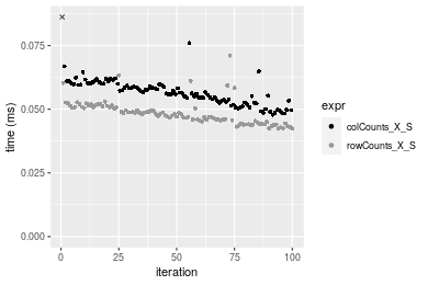
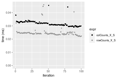
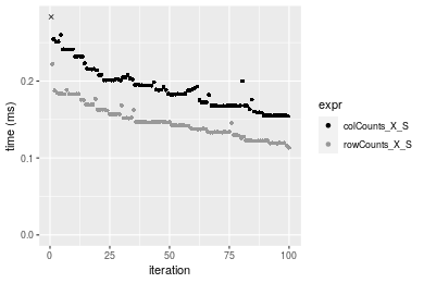
Figure: Benchmarking of colCounts_X_S() and rowCounts_X_S() on logical+100x100 data (original and transposed). Outliers are displayed as crosses. Times are in milliseconds.

1000x10 matrix

> X <- data[["1000x10"]]
> rows <- sample.int(nrow(X), size = nrow(X) * 0.7)
> cols <- sample.int(ncol(X), size = ncol(X) * 0.7)
> X_S <- X[rows, cols]
> value <- 42

> colStats <- microbenchmark(colCounts_X_S = colCounts(X_S, value = value, na.rm = FALSE), `colCounts(X, rows, cols)` = colCounts(X, 
+     value = value, na.rm = FALSE, rows = rows, cols = cols), `colCounts(X[rows, cols])` = colCounts(X[rows, 
+     cols], value = value, na.rm = FALSE), unit = "ms")

> X <- t(X)
> X_S <- t(X_S)

> rowStats <- microbenchmark(rowCounts_X_S = rowCounts(X_S, value = value, na.rm = FALSE), `rowCounts(X, cols, rows)` = rowCounts(X, 
+     value = value, na.rm = FALSE, rows = cols, cols = rows), `rowCounts(X[cols, rows])` = rowCounts(X[cols, 
+     rows], value = value, na.rm = FALSE), unit = "ms")

Table: Benchmarking of colCounts_X_S(), colCounts(X, rows, cols)() and colCounts(X[rows, cols])() on logical+1000x10 data. The top panel shows times in milliseconds and the bottom panel shows relative times.

	expr	min	lq	mean	median	uq	max
1	colCounts_X_S	0.045959	0.0501845	0.0520615	0.052198	0.0542395	0.062869
2	colCounts(X, rows, cols)	0.045529	0.0494745	0.0530975	0.053281	0.0558440	0.067862
3	colCounts(X[rows, cols])	0.059861	0.0621925	0.0680622	0.067737	0.0717325	0.124888

	expr	min	lq	mean	median	uq	max
1	colCounts_X_S	1.0000000	1.0000000	1.000000	1.000000	1.000000	1.000000
2	colCounts(X, rows, cols)	0.9906438	0.9858522	1.019900	1.020748	1.029582	1.079419
3	colCounts(X[rows, cols])	1.3024870	1.2392771	1.307343	1.297693	1.322514	1.986480

Table: Benchmarking of rowCounts_X_S(), rowCounts(X, cols, rows)() and rowCounts(X[cols, rows])() on logical+1000x10 data (transposed). The top panel shows times in milliseconds and the bottom panel shows relative times.

	expr	min	lq	mean	median	uq	max
1	rowCounts_X_S	0.043776	0.0460805	0.0500111	0.0476390	0.0527105	0.083305
2	rowCounts(X, cols, rows)	0.050551	0.0556310	0.0592041	0.0590905	0.0624135	0.072089
3	rowCounts(X[cols, rows])	0.059092	0.0629215	0.0683959	0.0673615	0.0724645	0.140307

	expr	min	lq	mean	median	uq	max
1	rowCounts_X_S	1.000000	1.000000	1.000000	1.000000	1.000000	1.0000000
2	rowCounts(X, cols, rows)	1.154765	1.207257	1.183818	1.240381	1.184081	0.8653622
3	rowCounts(X[cols, rows])	1.349872	1.365469	1.367614	1.413999	1.374764	1.6842566

Figure: Benchmarking of colCounts_X_S(), colCounts(X, rows, cols)() and colCounts(X[rows, cols])() on logical+1000x10 data as well as rowCounts_X_S(), rowCounts(X, cols, rows)() and rowCounts(X[cols, rows])() on the same data transposed. Outliers are displayed as crosses. Times are in milliseconds.

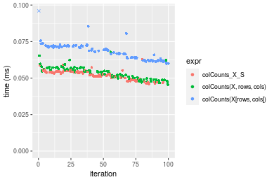
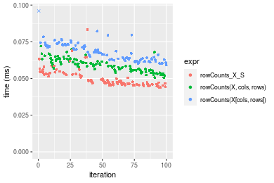Table: Benchmarking of colCounts_X_S() and rowCounts_X_S() on logical+1000x10 data (original and transposed). The top panel shows times in milliseconds and the bottom panel shows relative times.

	expr	min	lq	mean	median	uq	max
2	rowCounts_X_S	43.776	46.0805	50.01115	47.639	52.7105	83.305
1	colCounts_X_S	45.959	50.1845	52.06151	52.198	54.2395	62.869

	expr	min	lq	mean	median	uq	max
2	rowCounts_X_S	1.000000	1.000000	1.000000	1.000000	1.000000	1.0000000
1	colCounts_X_S	1.049867	1.089061	1.040998	1.095699	1.029008	0.7546846

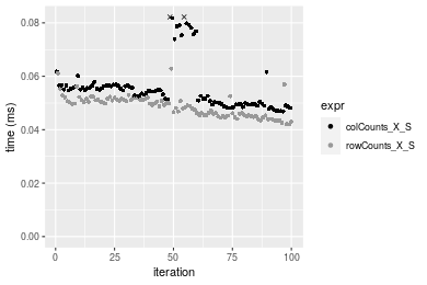
Figure: Benchmarking of colCounts_X_S() and rowCounts_X_S() on logical+1000x10 data (original and transposed). Outliers are displayed as crosses. Times are in milliseconds.

10x1000 matrix

> X <- data[["10x1000"]]
> rows <- sample.int(nrow(X), size = nrow(X) * 0.7)
> cols <- sample.int(ncol(X), size = ncol(X) * 0.7)
> X_S <- X[rows, cols]
> value <- 42

> colStats <- microbenchmark(colCounts_X_S = colCounts(X_S, value = value, na.rm = FALSE), `colCounts(X, rows, cols)` = colCounts(X, 
+     value = value, na.rm = FALSE, rows = rows, cols = cols), `colCounts(X[rows, cols])` = colCounts(X[rows, 
+     cols], value = value, na.rm = FALSE), unit = "ms")

> X <- t(X)
> X_S <- t(X_S)

> rowStats <- microbenchmark(rowCounts_X_S = rowCounts(X_S, value = value, na.rm = FALSE), `rowCounts(X, cols, rows)` = rowCounts(X, 
+     value = value, na.rm = FALSE, rows = cols, cols = rows), `rowCounts(X[cols, rows])` = rowCounts(X[cols, 
+     rows], value = value, na.rm = FALSE), unit = "ms")

Table: Benchmarking of colCounts_X_S(), colCounts(X, rows, cols)() and colCounts(X[rows, cols])() on logical+10x1000 data. The top panel shows times in milliseconds and the bottom panel shows relative times.

	expr	min	lq	mean	median	uq	max
1	colCounts_X_S	0.047879	0.0531215	0.0569036	0.0566190	0.0598395	0.107495
2	colCounts(X, rows, cols)	0.052682	0.0560680	0.0610084	0.0594745	0.0654255	0.097622
3	colCounts(X[rows, cols])	0.063060	0.0705530	0.0742625	0.0740445	0.0785110	0.091614

	expr	min	lq	mean	median	uq	max
1	colCounts_X_S	1.000000	1.000000	1.000000	1.000000	1.000000	1.0000000
2	colCounts(X, rows, cols)	1.100315	1.055467	1.072136	1.050434	1.093350	0.9081539
3	colCounts(X[rows, cols])	1.317070	1.328144	1.305057	1.307768	1.312026	0.8522629

Table: Benchmarking of rowCounts_X_S(), rowCounts(X, cols, rows)() and rowCounts(X[cols, rows])() on logical+10x1000 data (transposed). The top panel shows times in milliseconds and the bottom panel shows relative times.

	expr	min	lq	mean	median	uq	max
1	rowCounts_X_S	0.042457	0.0453510	0.0484223	0.0480365	0.0507445	0.071069
2	rowCounts(X, cols, rows)	0.044221	0.0502810	0.0539310	0.0530740	0.0569600	0.107396
3	rowCounts(X[cols, rows])	0.056435	0.0605775	0.0644457	0.0640835	0.0688170	0.081165

	expr	min	lq	mean	median	uq	max
1	rowCounts_X_S	1.000000	1.000000	1.000000	1.000000	1.000000	1.000000
2	rowCounts(X, cols, rows)	1.041548	1.108708	1.113765	1.104868	1.122486	1.511151
3	rowCounts(X[cols, rows])	1.329227	1.335748	1.330909	1.334059	1.356147	1.142059

Figure: Benchmarking of colCounts_X_S(), colCounts(X, rows, cols)() and colCounts(X[rows, cols])() on logical+10x1000 data as well as rowCounts_X_S(), rowCounts(X, cols, rows)() and rowCounts(X[cols, rows])() on the same data transposed. Outliers are displayed as crosses. Times are in milliseconds.

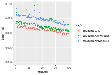
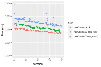Table: Benchmarking of colCounts_X_S() and rowCounts_X_S() on logical+10x1000 data (original and transposed). The top panel shows times in milliseconds and the bottom panel shows relative times.

	expr	min	lq	mean	median	uq	max
2	rowCounts_X_S	42.457	45.3510	48.42229	48.0365	50.7445	71.069
1	colCounts_X_S	47.879	53.1215	56.90362	56.6190	59.8395	107.495

	expr	min	lq	mean	median	uq	max
2	rowCounts_X_S	1.000000	1.000000	1.000000	1.000000	1.000000	1.000000
1	colCounts_X_S	1.127706	1.171341	1.175153	1.178666	1.179231	1.512544

Figure: Benchmarking of colCounts_X_S() and rowCounts_X_S() on logical+10x1000 data (original and transposed). Outliers are displayed as crosses. Times are in milliseconds.

100x1000 matrix

> X <- data[["100x1000"]]
> rows <- sample.int(nrow(X), size = nrow(X) * 0.7)
> cols <- sample.int(ncol(X), size = ncol(X) * 0.7)
> X_S <- X[rows, cols]
> value <- 42

> colStats <- microbenchmark(colCounts_X_S = colCounts(X_S, value = value, na.rm = FALSE), `colCounts(X, rows, cols)` = colCounts(X, 
+     value = value, na.rm = FALSE, rows = rows, cols = cols), `colCounts(X[rows, cols])` = colCounts(X[rows, 
+     cols], value = value, na.rm = FALSE), unit = "ms")

> X <- t(X)
> X_S <- t(X_S)

> rowStats <- microbenchmark(rowCounts_X_S = rowCounts(X_S, value = value, na.rm = FALSE), `rowCounts(X, cols, rows)` = rowCounts(X, 
+     value = value, na.rm = FALSE, rows = cols, cols = rows), `rowCounts(X[cols, rows])` = rowCounts(X[cols, 
+     rows], value = value, na.rm = FALSE), unit = "ms")

Table: Benchmarking of colCounts_X_S(), colCounts(X, rows, cols)() and colCounts(X[rows, cols])() on logical+100x1000 data. The top panel shows times in milliseconds and the bottom panel shows relative times.

	expr	min	lq	mean	median	uq	max
1	colCounts_X_S	0.298485	0.2996055	0.3339752	0.3009455	0.3594510	0.530982
2	colCounts(X, rows, cols)	0.299571	0.3013045	0.3356421	0.3037735	0.3708485	0.558535
3	colCounts(X[rows, cols])	0.390523	0.3921000	0.4410802	0.3957280	0.4719525	0.646900

	expr	min	lq	mean	median	uq	max
1	colCounts_X_S	1.000000	1.000000	1.000000	1.000000	1.000000	1.000000
2	colCounts(X, rows, cols)	1.003638	1.005671	1.004991	1.009397	1.031708	1.051891
3	colCounts(X[rows, cols])	1.308350	1.308721	1.320697	1.314949	1.312982	1.218309

Table: Benchmarking of rowCounts_X_S(), rowCounts(X, cols, rows)() and rowCounts(X[cols, rows])() on logical+100x1000 data (transposed). The top panel shows times in milliseconds and the bottom panel shows relative times.

	expr	min	lq	mean	median	uq	max
1	rowCounts_X_S	0.283070	0.2850815	0.3246799	0.291610	0.3480445	0.501973
2	rowCounts(X, cols, rows)	0.308049	0.3094795	0.3364997	0.310451	0.3459055	0.541672
3	rowCounts(X[cols, rows])	0.374334	0.3766000	0.4194284	0.379685	0.4538615	0.622969

	expr	min	lq	mean	median	uq	max
1	rowCounts_X_S	1.000000	1.000000	1.000000	1.00000	1.0000000	1.000000
2	rowCounts(X, cols, rows)	1.088243	1.085582	1.036404	1.06461	0.9938542	1.079086
3	rowCounts(X[cols, rows])	1.322408	1.321026	1.291821	1.30203	1.3040330	1.241041

Figure: Benchmarking of colCounts_X_S(), colCounts(X, rows, cols)() and colCounts(X[rows, cols])() on logical+100x1000 data as well as rowCounts_X_S(), rowCounts(X, cols, rows)() and rowCounts(X[cols, rows])() on the same data transposed. Outliers are displayed as crosses. Times are in milliseconds.

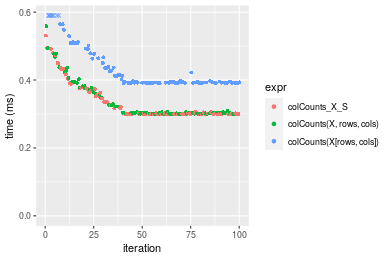
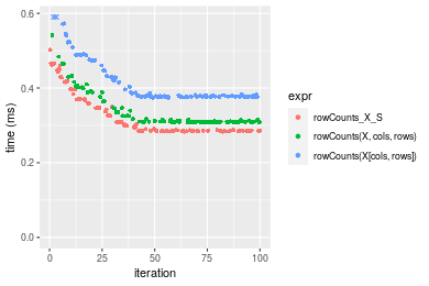Table: Benchmarking of colCounts_X_S() and rowCounts_X_S() on logical+100x1000 data (original and transposed). The top panel shows times in milliseconds and the bottom panel shows relative times.

	expr	min	lq	mean	median	uq	max
2	rowCounts_X_S	283.070	285.0815	324.6799	291.6100	348.0445	501.973
1	colCounts_X_S	298.485	299.6055	333.9752	300.9455	359.4510	530.982

	expr	min	lq	mean	median	uq	max
2	rowCounts_X_S	1.000000	1.000000	1.000000	1.000000	1.000000	1.00000
1	colCounts_X_S	1.054456	1.050947	1.028629	1.032014	1.032773	1.05779

Figure: Benchmarking of colCounts_X_S() and rowCounts_X_S() on logical+100x1000 data (original and transposed). Outliers are displayed as crosses. Times are in milliseconds.

1000x100 matrix

> X <- data[["1000x100"]]
> rows <- sample.int(nrow(X), size = nrow(X) * 0.7)
> cols <- sample.int(ncol(X), size = ncol(X) * 0.7)
> X_S <- X[rows, cols]
> value <- 42

> colStats <- microbenchmark(colCounts_X_S = colCounts(X_S, value = value, na.rm = FALSE), `colCounts(X, rows, cols)` = colCounts(X, 
+     value = value, na.rm = FALSE, rows = rows, cols = cols), `colCounts(X[rows, cols])` = colCounts(X[rows, 
+     cols], value = value, na.rm = FALSE), unit = "ms")

> X <- t(X)
> X_S <- t(X_S)

> rowStats <- microbenchmark(rowCounts_X_S = rowCounts(X_S, value = value, na.rm = FALSE), `rowCounts(X, cols, rows)` = rowCounts(X, 
+     value = value, na.rm = FALSE, rows = cols, cols = rows), `rowCounts(X[cols, rows])` = rowCounts(X[cols, 
+     rows], value = value, na.rm = FALSE), unit = "ms")

Table: Benchmarking of colCounts_X_S(), colCounts(X, rows, cols)() and colCounts(X[rows, cols])() on logical+1000x100 data. The top panel shows times in milliseconds and the bottom panel shows relative times.

	expr	min	lq	mean	median	uq	max
1	colCounts_X_S	0.291383	0.2924520	0.3234710	0.2935325	0.3222405	0.526776
2	colCounts(X, rows, cols)	0.291557	0.2933380	0.3328575	0.3009670	0.3535535	0.484701
3	colCounts(X[rows, cols])	0.383425	0.3850015	0.4350638	0.3935370	0.4842905	0.678262

	expr	min	lq	mean	median	uq	max
1	colCounts_X_S	1.000000	1.000000	1.000000	1.000000	1.000000	1.0000000
2	colCounts(X, rows, cols)	1.000597	1.003030	1.029018	1.025328	1.097173	0.9201273
3	colCounts(X[rows, cols])	1.315880	1.316461	1.344985	1.340693	1.502885	1.2875719

Table: Benchmarking of rowCounts_X_S(), rowCounts(X, cols, rows)() and rowCounts(X[cols, rows])() on logical+1000x100 data (transposed). The top panel shows times in milliseconds and the bottom panel shows relative times.

	expr	min	lq	mean	median	uq	max
1	rowCounts_X_S	0.286594	0.2891705	0.3219671	0.2916335	0.3501715	0.481144
2	rowCounts(X, cols, rows)	0.315138	0.3168990	0.3534171	0.3182890	0.3746905	0.604319
3	rowCounts(X[cols, rows])	0.378691	0.3820230	0.4257085	0.3867375	0.4666055	0.631997

	expr	min	lq	mean	median	uq	max
1	rowCounts_X_S	1.000000	1.00000	1.000000	1.000000	1.000000	1.000000
2	rowCounts(X, cols, rows)	1.099597	1.09589	1.097681	1.091401	1.070020	1.256004
3	rowCounts(X[cols, rows])	1.321350	1.32110	1.322211	1.326108	1.332506	1.313530

Figure: Benchmarking of colCounts_X_S(), colCounts(X, rows, cols)() and colCounts(X[rows, cols])() on logical+1000x100 data as well as rowCounts_X_S(), rowCounts(X, cols, rows)() and rowCounts(X[cols, rows])() on the same data transposed. Outliers are displayed as crosses. Times are in milliseconds.

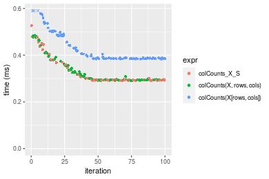
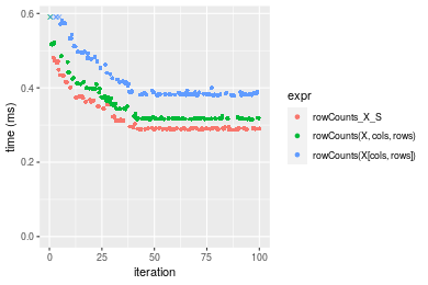Table: Benchmarking of colCounts_X_S() and rowCounts_X_S() on logical+1000x100 data (original and transposed). The top panel shows times in milliseconds and the bottom panel shows relative times.

	expr	min	lq	mean	median	uq	max
2	rowCounts_X_S	286.594	289.1705	321.9671	291.6335	350.1715	481.144
1	colCounts_X_S	291.383	292.4520	323.4710	293.5325	322.2405	526.776

	expr	min	lq	mean	median	uq	max
2	rowCounts_X_S	1.00000	1.000000	1.000000	1.000000	1.0000000	1.000000
1	colCounts_X_S	1.01671	1.011348	1.004671	1.006512	0.9202362	1.094841

Figure: Benchmarking of colCounts_X_S() and rowCounts_X_S() on logical+1000x100 data (original and transposed). Outliers are displayed as crosses. Times are in milliseconds.

Data type “integer”

Data

> rmatrix <- function(nrow, ncol, mode = c("logical", "double", "integer", "index"), range = c(-100, 
+     +100), na_prob = 0) {
+     mode <- match.arg(mode)
+     n <- nrow * ncol
+     if (mode == "logical") {
+         x <- sample(c(FALSE, TRUE), size = n, replace = TRUE)
+     }     else if (mode == "index") {
+         x <- seq_len(n)
+         mode <- "integer"
+     }     else {
+         x <- runif(n, min = range[1], max = range[2])
+     }
+     storage.mode(x) <- mode
+     if (na_prob > 0) 
+         x[sample(n, size = na_prob * n)] <- NA
+     dim(x) <- c(nrow, ncol)
+     x
+ }
> rmatrices <- function(scale = 10, seed = 1, ...) {
+     set.seed(seed)
+     data <- list()
+     data[[1]] <- rmatrix(nrow = scale * 1, ncol = scale * 1, ...)
+     data[[2]] <- rmatrix(nrow = scale * 10, ncol = scale * 10, ...)
+     data[[3]] <- rmatrix(nrow = scale * 100, ncol = scale * 1, ...)
+     data[[4]] <- t(data[[3]])
+     data[[5]] <- rmatrix(nrow = scale * 10, ncol = scale * 100, ...)
+     data[[6]] <- t(data[[5]])
+     names(data) <- sapply(data, FUN = function(x) paste(dim(x), collapse = "x"))
+     data
+ }
> data <- rmatrices(mode = mode)

Results

10x10 matrix

> X <- data[["10x10"]]
> rows <- sample.int(nrow(X), size = nrow(X) * 0.7)
> cols <- sample.int(ncol(X), size = ncol(X) * 0.7)
> X_S <- X[rows, cols]
> value <- 42

> colStats <- microbenchmark(colCounts_X_S = colCounts(X_S, value = value, na.rm = FALSE), `colCounts(X, rows, cols)` = colCounts(X, 
+     value = value, na.rm = FALSE, rows = rows, cols = cols), `colCounts(X[rows, cols])` = colCounts(X[rows, 
+     cols], value = value, na.rm = FALSE), unit = "ms")

> X <- t(X)
> X_S <- t(X_S)

> rowStats <- microbenchmark(rowCounts_X_S = rowCounts(X_S, value = value, na.rm = FALSE), `rowCounts(X, cols, rows)` = rowCounts(X, 
+     value = value, na.rm = FALSE, rows = cols, cols = rows), `rowCounts(X[cols, rows])` = rowCounts(X[cols, 
+     rows], value = value, na.rm = FALSE), unit = "ms")

Table: Benchmarking of colCounts_X_S(), colCounts(X, rows, cols)() and colCounts(X[rows, cols])() on integer+10x10 data. The top panel shows times in milliseconds and the bottom panel shows relative times.

	expr	min	lq	mean	median	uq	max
1	colCounts_X_S	0.007935	0.0082455	0.0088977	0.0083860	0.0084945	0.050990
2	colCounts(X, rows, cols)	0.008451	0.0086965	0.0088557	0.0088080	0.0089420	0.011728
3	colCounts(X[rows, cols])	0.009318	0.0097190	0.0100383	0.0099555	0.0101355	0.016553

	expr	min	lq	mean	median	uq	max
1	colCounts_X_S	1.000000	1.000000	1.0000000	1.000000	1.000000	1.0000000
2	colCounts(X, rows, cols)	1.065028	1.054696	0.9952808	1.050322	1.052681	0.2300059
3	colCounts(X[rows, cols])	1.174291	1.178703	1.1281963	1.187157	1.193184	0.3246323

Table: Benchmarking of rowCounts_X_S(), rowCounts(X, cols, rows)() and rowCounts(X[cols, rows])() on integer+10x10 data (transposed). The top panel shows times in milliseconds and the bottom panel shows relative times.

	expr	min	lq	mean	median	uq	max
1	rowCounts_X_S	0.006826	0.0069965	0.0071737	0.0071190	0.0072425	0.010086
2	rowCounts(X, cols, rows)	0.007208	0.0073815	0.0080176	0.0074885	0.0076930	0.048277
3	rowCounts(X[cols, rows])	0.008005	0.0083720	0.0086312	0.0085180	0.0087065	0.013023

	expr	min	lq	mean	median	uq	max
1	rowCounts_X_S	1.000000	1.000000	1.000000	1.000000	1.000000	1.000000
2	rowCounts(X, cols, rows)	1.055962	1.055028	1.117632	1.051903	1.062202	4.786536
3	rowCounts(X[cols, rows])	1.172722	1.196598	1.203177	1.196516	1.202140	1.291196

Figure: Benchmarking of colCounts_X_S(), colCounts(X, rows, cols)() and colCounts(X[rows, cols])() on integer+10x10 data as well as rowCounts_X_S(), rowCounts(X, cols, rows)() and rowCounts(X[cols, rows])() on the same data transposed. Outliers are displayed as crosses. Times are in milliseconds.

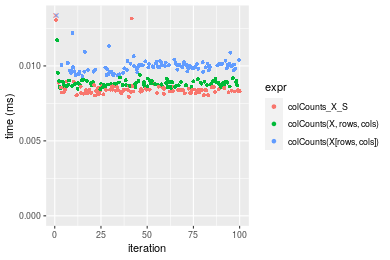
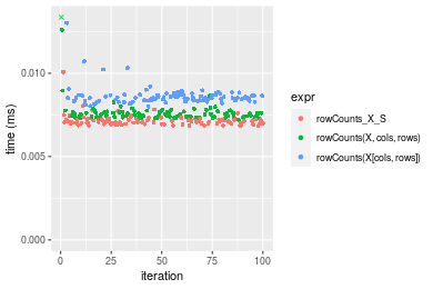Table: Benchmarking of colCounts_X_S() and rowCounts_X_S() on integer+10x10 data (original and transposed). The top panel shows times in milliseconds and the bottom panel shows relative times.

	expr	min	lq	mean	median	uq	max
2	rowCounts_X_S	6.826	6.9965	7.17371	7.119	7.2425	10.086
1	colCounts_X_S	7.935	8.2455	8.89768	8.386	8.4945	50.990

	expr	min	lq	mean	median	uq	max
2	rowCounts_X_S	1.000000	1.000000	1.000000	1.000000	1.000000	1.000000
1	colCounts_X_S	1.162467	1.178518	1.240318	1.177974	1.172869	5.055523

Figure: Benchmarking of colCounts_X_S() and rowCounts_X_S() on integer+10x10 data (original and transposed). Outliers are displayed as crosses. Times are in milliseconds.

100x100 matrix

> X <- data[["100x100"]]
> rows <- sample.int(nrow(X), size = nrow(X) * 0.7)
> cols <- sample.int(ncol(X), size = ncol(X) * 0.7)
> X_S <- X[rows, cols]
> value <- 42

> colStats <- microbenchmark(colCounts_X_S = colCounts(X_S, value = value, na.rm = FALSE), `colCounts(X, rows, cols)` = colCounts(X, 
+     value = value, na.rm = FALSE, rows = rows, cols = cols), `colCounts(X[rows, cols])` = colCounts(X[rows, 
+     cols], value = value, na.rm = FALSE), unit = "ms")

> X <- t(X)
> X_S <- t(X_S)

> rowStats <- microbenchmark(rowCounts_X_S = rowCounts(X_S, value = value, na.rm = FALSE), `rowCounts(X, cols, rows)` = rowCounts(X, 
+     value = value, na.rm = FALSE, rows = cols, cols = rows), `rowCounts(X[cols, rows])` = rowCounts(X[cols, 
+     rows], value = value, na.rm = FALSE), unit = "ms")

Table: Benchmarking of colCounts_X_S(), colCounts(X, rows, cols)() and colCounts(X[rows, cols])() on integer+100x100 data. The top panel shows times in milliseconds and the bottom panel shows relative times.

	expr	min	lq	mean	median	uq	max
2	colCounts(X, rows, cols)	0.026692	0.0280625	0.0292683	0.0287570	0.030393	0.044949
1	colCounts_X_S	0.029141	0.0305555	0.0318885	0.0318105	0.033061	0.045509
3	colCounts(X[rows, cols])	0.040022	0.0416785	0.0441608	0.0433700	0.045669	0.106045

	expr	min	lq	mean	median	uq	max
2	colCounts(X, rows, cols)	1.000000	1.000000	1.000000	1.000000	1.000000	1.000000
1	colCounts_X_S	1.091750	1.088837	1.089525	1.106183	1.087783	1.012459
3	colCounts(X[rows, cols])	1.499401	1.485203	1.508830	1.508155	1.502616	2.359229

Table: Benchmarking of rowCounts_X_S(), rowCounts(X, cols, rows)() and rowCounts(X[cols, rows])() on integer+100x100 data (transposed). The top panel shows times in milliseconds and the bottom panel shows relative times.

	expr	min	lq	mean	median	uq	max
1	rowCounts_X_S	0.022066	0.0237195	0.0251630	0.0242375	0.0249070	0.046011
2	rowCounts(X, cols, rows)	0.023473	0.0252140	0.0276956	0.0254965	0.0265005	0.074319
3	rowCounts(X[cols, rows])	0.032393	0.0348880	0.0380130	0.0357730	0.0373220	0.068968

	expr	min	lq	mean	median	uq	max
1	rowCounts_X_S	1.000000	1.000000	1.000000	1.000000	1.000000	1.000000
2	rowCounts(X, cols, rows)	1.063763	1.063007	1.100648	1.051944	1.063978	1.615244
3	rowCounts(X[cols, rows])	1.468005	1.470857	1.510668	1.475936	1.498454	1.498946

Figure: Benchmarking of colCounts_X_S(), colCounts(X, rows, cols)() and colCounts(X[rows, cols])() on integer+100x100 data as well as rowCounts_X_S(), rowCounts(X, cols, rows)() and rowCounts(X[cols, rows])() on the same data transposed. Outliers are displayed as crosses. Times are in milliseconds.

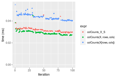
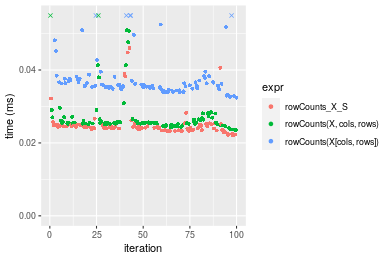Table: Benchmarking of colCounts_X_S() and rowCounts_X_S() on integer+100x100 data (original and transposed). The top panel shows times in milliseconds and the bottom panel shows relative times.

	expr	min	lq	mean	median	uq	max
2	rowCounts_X_S	22.066	23.7195	25.16304	24.2375	24.907	46.011
1	colCounts_X_S	29.141	30.5555	31.88851	31.8105	33.061	45.509

	expr	min	lq	mean	median	uq	max
2	rowCounts_X_S	1.000000	1.000000	1.000000	1.00000	1.000000	1.0000000
1	colCounts_X_S	1.320629	1.288202	1.267276	1.31245	1.327378	0.9890896

Figure: Benchmarking of colCounts_X_S() and rowCounts_X_S() on integer+100x100 data (original and transposed). Outliers are displayed as crosses. Times are in milliseconds.

1000x10 matrix

> X <- data[["1000x10"]]
> rows <- sample.int(nrow(X), size = nrow(X) * 0.7)
> cols <- sample.int(ncol(X), size = ncol(X) * 0.7)
> X_S <- X[rows, cols]
> value <- 42

> colStats <- microbenchmark(colCounts_X_S = colCounts(X_S, value = value, na.rm = FALSE), `colCounts(X, rows, cols)` = colCounts(X, 
+     value = value, na.rm = FALSE, rows = rows, cols = cols), `colCounts(X[rows, cols])` = colCounts(X[rows, 
+     cols], value = value, na.rm = FALSE), unit = "ms")

> X <- t(X)
> X_S <- t(X_S)

> rowStats <- microbenchmark(rowCounts_X_S = rowCounts(X_S, value = value, na.rm = FALSE), `rowCounts(X, cols, rows)` = rowCounts(X, 
+     value = value, na.rm = FALSE, rows = cols, cols = rows), `rowCounts(X[cols, rows])` = rowCounts(X[cols, 
+     rows], value = value, na.rm = FALSE), unit = "ms")

Table: Benchmarking of colCounts_X_S(), colCounts(X, rows, cols)() and colCounts(X[rows, cols])() on integer+1000x10 data. The top panel shows times in milliseconds and the bottom panel shows relative times.

	expr	min	lq	mean	median	uq	max
2	colCounts(X, rows, cols)	0.027454	0.028800	0.0304023	0.0299545	0.0313025	0.043183
1	colCounts_X_S	0.027870	0.029747	0.0309909	0.0313055	0.0316895	0.045871
3	colCounts(X[rows, cols])	0.039156	0.041092	0.0434713	0.0428355	0.0446275	0.099119

	expr	min	lq	mean	median	uq	max
2	colCounts(X, rows, cols)	1.000000	1.000000	1.000000	1.000000	1.000000	1.000000
1	colCounts_X_S	1.015153	1.032882	1.019361	1.045102	1.012363	1.062247
3	colCounts(X[rows, cols])	1.426240	1.426806	1.429870	1.430019	1.425685	2.295324

Table: Benchmarking of rowCounts_X_S(), rowCounts(X, cols, rows)() and rowCounts(X[cols, rows])() on integer+1000x10 data (transposed). The top panel shows times in milliseconds and the bottom panel shows relative times.

	expr	min	lq	mean	median	uq	max
1	rowCounts_X_S	0.026430	0.0267475	0.0297994	0.0271785	0.0278660	0.075157
2	rowCounts(X, cols, rows)	0.029471	0.0301460	0.0349535	0.0312645	0.0339875	0.070251
3	rowCounts(X[cols, rows])	0.040792	0.0415505	0.0469084	0.0423595	0.0476420	0.101546

	expr	min	lq	mean	median	uq	max
1	rowCounts_X_S	1.000000	1.000000	1.000000	1.000000	1.000000	1.0000000
2	rowCounts(X, cols, rows)	1.115059	1.127059	1.172960	1.150339	1.219676	0.9347233
3	rowCounts(X[cols, rows])	1.543398	1.553435	1.574139	1.558566	1.709682	1.3511183

Figure: Benchmarking of colCounts_X_S(), colCounts(X, rows, cols)() and colCounts(X[rows, cols])() on integer+1000x10 data as well as rowCounts_X_S(), rowCounts(X, cols, rows)() and rowCounts(X[cols, rows])() on the same data transposed. Outliers are displayed as crosses. Times are in milliseconds.

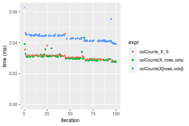
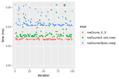Table: Benchmarking of colCounts_X_S() and rowCounts_X_S() on integer+1000x10 data (original and transposed). The top panel shows times in milliseconds and the bottom panel shows relative times.

	expr	min	lq	mean	median	uq	max
2	rowCounts_X_S	26.43	26.7475	29.79937	27.1785	27.8660	75.157
1	colCounts_X_S	27.87	29.7470	30.99093	31.3055	31.6895	45.871

	expr	min	lq	mean	median	uq	max
2	rowCounts_X_S	1.000000	1.000000	1.000000	1.000000	1.00000	1.0000000
1	colCounts_X_S	1.054483	1.112141	1.039986	1.151848	1.13721	0.6103357

Figure: Benchmarking of colCounts_X_S() and rowCounts_X_S() on integer+1000x10 data (original and transposed). Outliers are displayed as crosses. Times are in milliseconds.

10x1000 matrix

> X <- data[["10x1000"]]
> rows <- sample.int(nrow(X), size = nrow(X) * 0.7)
> cols <- sample.int(ncol(X), size = ncol(X) * 0.7)
> X_S <- X[rows, cols]
> value <- 42

> colStats <- microbenchmark(colCounts_X_S = colCounts(X_S, value = value, na.rm = FALSE), `colCounts(X, rows, cols)` = colCounts(X, 
+     value = value, na.rm = FALSE, rows = rows, cols = cols), `colCounts(X[rows, cols])` = colCounts(X[rows, 
+     cols], value = value, na.rm = FALSE), unit = "ms")

> X <- t(X)
> X_S <- t(X_S)

> rowStats <- microbenchmark(rowCounts_X_S = rowCounts(X_S, value = value, na.rm = FALSE), `rowCounts(X, cols, rows)` = rowCounts(X, 
+     value = value, na.rm = FALSE, rows = cols, cols = rows), `rowCounts(X[cols, rows])` = rowCounts(X[cols, 
+     rows], value = value, na.rm = FALSE), unit = "ms")

Table: Benchmarking of colCounts_X_S(), colCounts(X, rows, cols)() and colCounts(X[rows, cols])() on integer+10x1000 data. The top panel shows times in milliseconds and the bottom panel shows relative times.

	expr	min	lq	mean	median	uq	max
2	colCounts(X, rows, cols)	0.030790	0.0317475	0.0331242	0.0328270	0.0340955	0.050668
1	colCounts_X_S	0.032081	0.0333615	0.0353125	0.0350675	0.0364430	0.078019
3	colCounts(X[rows, cols])	0.045466	0.0477120	0.0499071	0.0495685	0.0515210	0.064295

	expr	min	lq	mean	median	uq	max
2	colCounts(X, rows, cols)	1.000000	1.000000	1.000000	1.000000	1.000000	1.000000
1	colCounts_X_S	1.041929	1.050839	1.066062	1.068252	1.068851	1.539808
3	colCounts(X[rows, cols])	1.476648	1.502859	1.506663	1.509992	1.511079	1.268947

Table: Benchmarking of rowCounts_X_S(), rowCounts(X, cols, rows)() and rowCounts(X[cols, rows])() on integer+10x1000 data (transposed). The top panel shows times in milliseconds and the bottom panel shows relative times.

	expr	min	lq	mean	median	uq	max
1	rowCounts_X_S	0.023672	0.0253500	0.0258507	0.0256975	0.0258715	0.039292
2	rowCounts(X, cols, rows)	0.026869	0.0276940	0.0289910	0.0284665	0.0286935	0.081112
3	rowCounts(X[cols, rows])	0.035510	0.0378125	0.0387588	0.0385730	0.0389335	0.053797

	expr	min	lq	mean	median	uq	max
1	rowCounts_X_S	1.000000	1.000000	1.000000	1.000000	1.000000	1.000000
2	rowCounts(X, cols, rows)	1.135054	1.092466	1.121477	1.107754	1.109078	2.064339
3	rowCounts(X[cols, rows])	1.500085	1.491617	1.499332	1.501041	1.504880	1.369159

Figure: Benchmarking of colCounts_X_S(), colCounts(X, rows, cols)() and colCounts(X[rows, cols])() on integer+10x1000 data as well as rowCounts_X_S(), rowCounts(X, cols, rows)() and rowCounts(X[cols, rows])() on the same data transposed. Outliers are displayed as crosses. Times are in milliseconds.

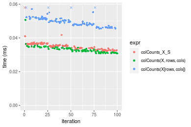
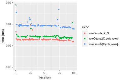Table: Benchmarking of colCounts_X_S() and rowCounts_X_S() on integer+10x1000 data (original and transposed). The top panel shows times in milliseconds and the bottom panel shows relative times.

	expr	min	lq	mean	median	uq	max
2	rowCounts_X_S	23.672	25.3500	25.85075	25.6975	25.8715	39.292
1	colCounts_X_S	32.081	33.3615	35.31249	35.0675	36.4430	78.019

	expr	min	lq	mean	median	uq	max
2	rowCounts_X_S	1.00000	1.000000	1.000000	1.000000	1.000000	1.000000
1	colCounts_X_S	1.35523	1.316035	1.366014	1.364627	1.408616	1.985621

Figure: Benchmarking of colCounts_X_S() and rowCounts_X_S() on integer+10x1000 data (original and transposed). Outliers are displayed as crosses. Times are in milliseconds.

100x1000 matrix

> X <- data[["100x1000"]]
> rows <- sample.int(nrow(X), size = nrow(X) * 0.7)
> cols <- sample.int(ncol(X), size = ncol(X) * 0.7)
> X_S <- X[rows, cols]
> value <- 42

> colStats <- microbenchmark(colCounts_X_S = colCounts(X_S, value = value, na.rm = FALSE), `colCounts(X, rows, cols)` = colCounts(X, 
+     value = value, na.rm = FALSE, rows = rows, cols = cols), `colCounts(X[rows, cols])` = colCounts(X[rows, 
+     cols], value = value, na.rm = FALSE), unit = "ms")

> X <- t(X)
> X_S <- t(X_S)

> rowStats <- microbenchmark(rowCounts_X_S = rowCounts(X_S, value = value, na.rm = FALSE), `rowCounts(X, cols, rows)` = rowCounts(X, 
+     value = value, na.rm = FALSE, rows = cols, cols = rows), `rowCounts(X[cols, rows])` = rowCounts(X[cols, 
+     rows], value = value, na.rm = FALSE), unit = "ms")

Table: Benchmarking of colCounts_X_S(), colCounts(X, rows, cols)() and colCounts(X[rows, cols])() on integer+100x1000 data. The top panel shows times in milliseconds and the bottom panel shows relative times.

	expr	min	lq	mean	median	uq	max
2	colCounts(X, rows, cols)	0.131224	0.1425110	0.1637071	0.1606255	0.1747210	0.277656
1	colCounts_X_S	0.154590	0.1678500	0.1918588	0.1887955	0.2040050	0.293703
3	colCounts(X[rows, cols])	0.221437	0.2460625	0.2817724	0.2786320	0.3082485	0.370760

	expr	min	lq	mean	median	uq	max
2	colCounts(X, rows, cols)	1.000000	1.000000	1.000000	1.000000	1.000000	1.000000
1	colCounts_X_S	1.178062	1.177804	1.171963	1.175377	1.167604	1.057794
3	colCounts(X[rows, cols])	1.687473	1.726621	1.721198	1.734668	1.764233	1.335321

Table: Benchmarking of rowCounts_X_S(), rowCounts(X, cols, rows)() and rowCounts(X[cols, rows])() on integer+100x1000 data (transposed). The top panel shows times in milliseconds and the bottom panel shows relative times.

	expr	min	lq	mean	median	uq	max
2	rowCounts(X, cols, rows)	0.115860	0.1252180	0.1403696	0.1370920	0.1498630	0.227246
1	rowCounts_X_S	0.113468	0.1332585	0.1471171	0.1458795	0.1620725	0.222371
3	rowCounts(X[cols, rows])	0.180713	0.2020355	0.2273156	0.2222070	0.2457760	0.298786

	expr	min	lq	mean	median	uq	max
2	rowCounts(X, cols, rows)	1.0000000	1.000000	1.000000	1.000000	1.000000	1.0000000
1	rowCounts_X_S	0.9793544	1.064212	1.048069	1.064099	1.081471	0.9785475
3	rowCounts(X[cols, rows])	1.5597532	1.613470	1.619407	1.620860	1.640005	1.3148130

Figure: Benchmarking of colCounts_X_S(), colCounts(X, rows, cols)() and colCounts(X[rows, cols])() on integer+100x1000 data as well as rowCounts_X_S(), rowCounts(X, cols, rows)() and rowCounts(X[cols, rows])() on the same data transposed. Outliers are displayed as crosses. Times are in milliseconds.

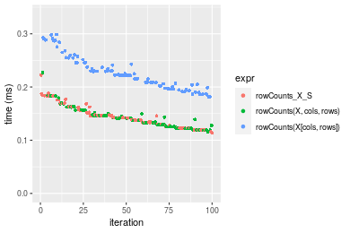Table: Benchmarking of colCounts_X_S() and rowCounts_X_S() on integer+100x1000 data (original and transposed). The top panel shows times in milliseconds and the bottom panel shows relative times.

	expr	min	lq	mean	median	uq	max
2	rowCounts_X_S	113.468	133.2585	147.1171	145.8795	162.0725	222.371
1	colCounts_X_S	154.590	167.8500	191.8587	188.7955	204.0050	293.703

	expr	min	lq	mean	median	uq	max
2	rowCounts_X_S	1.00000	1.000000	1.000000	1.000000	1.000000	1.000000
1	colCounts_X_S	1.36241	1.259582	1.304123	1.294188	1.258727	1.320779

Figure: Benchmarking of colCounts_X_S() and rowCounts_X_S() on integer+100x1000 data (original and transposed). Outliers are displayed as crosses. Times are in milliseconds.

1000x100 matrix

> X <- data[["1000x100"]]
> rows <- sample.int(nrow(X), size = nrow(X) * 0.7)
> cols <- sample.int(ncol(X), size = ncol(X) * 0.7)
> X_S <- X[rows, cols]
> value <- 42

> colStats <- microbenchmark(colCounts_X_S = colCounts(X_S, value = value, na.rm = FALSE), `colCounts(X, rows, cols)` = colCounts(X, 
+     value = value, na.rm = FALSE, rows = rows, cols = cols), `colCounts(X[rows, cols])` = colCounts(X[rows, 
+     cols], value = value, na.rm = FALSE), unit = "ms")

> X <- t(X)
> X_S <- t(X_S)

> rowStats <- microbenchmark(rowCounts_X_S = rowCounts(X_S, value = value, na.rm = FALSE), `rowCounts(X, cols, rows)` = rowCounts(X, 
+     value = value, na.rm = FALSE, rows = cols, cols = rows), `rowCounts(X[cols, rows])` = rowCounts(X[cols, 
+     rows], value = value, na.rm = FALSE), unit = "ms")

Table: Benchmarking of colCounts_X_S(), colCounts(X, rows, cols)() and colCounts(X[rows, cols])() on integer+1000x100 data. The top panel shows times in milliseconds and the bottom panel shows relative times.

	expr	min	lq	mean	median	uq	max
2	colCounts(X, rows, cols)	0.125200	0.1359420	0.1580321	0.1578650	0.1684815	0.215864
1	colCounts_X_S	0.147378	0.1578085	0.1820205	0.1749135	0.1922670	0.279674
3	colCounts(X[rows, cols])	0.211187	0.2287370	0.2672602	0.2637755	0.2949215	0.400076

	expr	min	lq	mean	median	uq	max
2	colCounts(X, rows, cols)	1.000000	1.000000	1.000000	1.000000	1.000000	1.000000
1	colCounts_X_S	1.177141	1.160852	1.151795	1.107994	1.141176	1.295603
3	colCounts(X[rows, cols])	1.686797	1.682607	1.691177	1.670893	1.750468	1.853371

Table: Benchmarking of rowCounts_X_S(), rowCounts(X, cols, rows)() and rowCounts(X[cols, rows])() on integer+1000x100 data (transposed). The top panel shows times in milliseconds and the bottom panel shows relative times.

	expr	min	lq	mean	median	uq	max
1	rowCounts_X_S	0.117146	0.1287240	0.1489846	0.1472150	0.1634295	0.201448
2	rowCounts(X, cols, rows)	0.119126	0.1363395	0.1550906	0.1500535	0.1663200	0.313826
3	rowCounts(X[cols, rows])	0.183672	0.2050615	0.2351304	0.2249520	0.2611940	0.368807

	expr	min	lq	mean	median	uq	max
1	rowCounts_X_S	1.000000	1.000000	1.000000	1.000000	1.000000	1.000000
2	rowCounts(X, cols, rows)	1.016902	1.059162	1.040984	1.019281	1.017686	1.557851
3	rowCounts(X[cols, rows])	1.567890	1.593032	1.578219	1.528051	1.598206	1.830780

Figure: Benchmarking of colCounts_X_S(), colCounts(X, rows, cols)() and colCounts(X[rows, cols])() on integer+1000x100 data as well as rowCounts_X_S(), rowCounts(X, cols, rows)() and rowCounts(X[cols, rows])() on the same data transposed. Outliers are displayed as crosses. Times are in milliseconds.

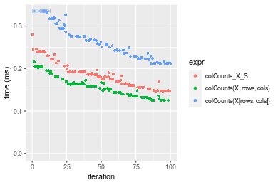
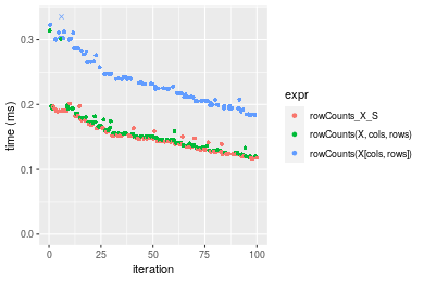Table: Benchmarking of colCounts_X_S() and rowCounts_X_S() on integer+1000x100 data (original and transposed). The top panel shows times in milliseconds and the bottom panel shows relative times.

	expr	min	lq	mean	median	uq	max
2	rowCounts_X_S	117.146	128.7240	148.9846	147.2150	163.4295	201.448
1	colCounts_X_S	147.378	157.8085	182.0205	174.9135	192.2670	279.674

	expr	min	lq	mean	median	uq	max
2	rowCounts_X_S	1.000000	1.000000	1.00000	1.00000	1.000000	1.000000
1	colCounts_X_S	1.258071	1.225945	1.22174	1.18815	1.176452	1.388319

Figure: Benchmarking of colCounts_X_S() and rowCounts_X_S() on integer+1000x100 data (original and transposed). Outliers are displayed as crosses. Times are in milliseconds.

Data type “double”

Data

> rmatrix <- function(nrow, ncol, mode = c("logical", "double", "integer", "index"), range = c(-100, 
+     +100), na_prob = 0) {
+     mode <- match.arg(mode)
+     n <- nrow * ncol
+     if (mode == "logical") {
+         x <- sample(c(FALSE, TRUE), size = n, replace = TRUE)
+     }     else if (mode == "index") {
+         x <- seq_len(n)
+         mode <- "integer"
+     }     else {
+         x <- runif(n, min = range[1], max = range[2])
+     }
+     storage.mode(x) <- mode
+     if (na_prob > 0) 
+         x[sample(n, size = na_prob * n)] <- NA
+     dim(x) <- c(nrow, ncol)
+     x
+ }
> rmatrices <- function(scale = 10, seed = 1, ...) {
+     set.seed(seed)
+     data <- list()
+     data[[1]] <- rmatrix(nrow = scale * 1, ncol = scale * 1, ...)
+     data[[2]] <- rmatrix(nrow = scale * 10, ncol = scale * 10, ...)
+     data[[3]] <- rmatrix(nrow = scale * 100, ncol = scale * 1, ...)
+     data[[4]] <- t(data[[3]])
+     data[[5]] <- rmatrix(nrow = scale * 10, ncol = scale * 100, ...)
+     data[[6]] <- t(data[[5]])
+     names(data) <- sapply(data, FUN = function(x) paste(dim(x), collapse = "x"))
+     data
+ }
> data <- rmatrices(mode = mode)

Results

10x10 matrix

> X <- data[["10x10"]]
> rows <- sample.int(nrow(X), size = nrow(X) * 0.7)
> cols <- sample.int(ncol(X), size = ncol(X) * 0.7)
> X_S <- X[rows, cols]
> value <- 42

> colStats <- microbenchmark(colCounts_X_S = colCounts(X_S, value = value, na.rm = FALSE), `colCounts(X, rows, cols)` = colCounts(X, 
+     value = value, na.rm = FALSE, rows = rows, cols = cols), `colCounts(X[rows, cols])` = colCounts(X[rows, 
+     cols], value = value, na.rm = FALSE), unit = "ms")

> X <- t(X)
> X_S <- t(X_S)

> rowStats <- microbenchmark(rowCounts_X_S = rowCounts(X_S, value = value, na.rm = FALSE), `rowCounts(X, cols, rows)` = rowCounts(X, 
+     value = value, na.rm = FALSE, rows = cols, cols = rows), `rowCounts(X[cols, rows])` = rowCounts(X[cols, 
+     rows], value = value, na.rm = FALSE), unit = "ms")

Table: Benchmarking of colCounts_X_S(), colCounts(X, rows, cols)() and colCounts(X[rows, cols])() on double+10x10 data. The top panel shows times in milliseconds and the bottom panel shows relative times.

	expr	min	lq	mean	median	uq	max
1	colCounts_X_S	0.007918	0.0081075	0.0086928	0.0082430	0.0083740	0.047964
2	colCounts(X, rows, cols)	0.008236	0.0085070	0.0086676	0.0085965	0.0087815	0.011631
3	colCounts(X[rows, cols])	0.009290	0.0096635	0.0099269	0.0098130	0.0100165	0.015073

	expr	min	lq	mean	median	uq	max
1	colCounts_X_S	1.000000	1.000000	1.0000000	1.000000	1.000000	1.0000000
2	colCounts(X, rows, cols)	1.040162	1.049275	0.9970907	1.042885	1.048663	0.2424944
3	colCounts(X[rows, cols])	1.173276	1.191921	1.1419582	1.190465	1.196143	0.3142565

Table: Benchmarking of rowCounts_X_S(), rowCounts(X, cols, rows)() and rowCounts(X[cols, rows])() on double+10x10 data (transposed). The top panel shows times in milliseconds and the bottom panel shows relative times.

	expr	min	lq	mean	median	uq	max
1	rowCounts_X_S	0.006889	0.0070615	0.0071825	0.0071215	0.0072670	0.010077
2	rowCounts(X, cols, rows)	0.007300	0.0074650	0.0080202	0.0075580	0.0077195	0.044605
3	rowCounts(X[cols, rows])	0.008122	0.0083415	0.0085558	0.0084855	0.0086460	0.011620

	expr	min	lq	mean	median	uq	max
1	rowCounts_X_S	1.000000	1.000000	1.000000	1.000000	1.000000	1.000000
2	rowCounts(X, cols, rows)	1.059660	1.057141	1.116631	1.061293	1.062268	4.426417
3	rowCounts(X[cols, rows])	1.178981	1.181265	1.191211	1.191533	1.189762	1.153121

Figure: Benchmarking of colCounts_X_S(), colCounts(X, rows, cols)() and colCounts(X[rows, cols])() on double+10x10 data as well as rowCounts_X_S(), rowCounts(X, cols, rows)() and rowCounts(X[cols, rows])() on the same data transposed. Outliers are displayed as crosses. Times are in milliseconds.

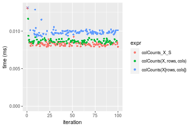
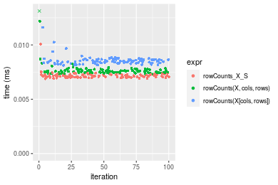Table: Benchmarking of colCounts_X_S() and rowCounts_X_S() on double+10x10 data (original and transposed). The top panel shows times in milliseconds and the bottom panel shows relative times.

	expr	min	lq	mean	median	uq	max
2	rowCounts_X_S	6.889	7.0615	7.18248	7.1215	7.267	10.077
1	colCounts_X_S	7.918	8.1075	8.69284	8.2430	8.374	47.964

	expr	min	lq	mean	median	uq	max
2	rowCounts_X_S	1.000000	1.000000	1.000000	1.000000	1.000000	1.00000
1	colCounts_X_S	1.149369	1.148127	1.210284	1.157481	1.152332	4.75975

Figure: Benchmarking of colCounts_X_S() and rowCounts_X_S() on double+10x10 data (original and transposed). Outliers are displayed as crosses. Times are in milliseconds.

100x100 matrix

> X <- data[["100x100"]]
> rows <- sample.int(nrow(X), size = nrow(X) * 0.7)
> cols <- sample.int(ncol(X), size = ncol(X) * 0.7)
> X_S <- X[rows, cols]
> value <- 42

> colStats <- microbenchmark(colCounts_X_S = colCounts(X_S, value = value, na.rm = FALSE), `colCounts(X, rows, cols)` = colCounts(X, 
+     value = value, na.rm = FALSE, rows = rows, cols = cols), `colCounts(X[rows, cols])` = colCounts(X[rows, 
+     cols], value = value, na.rm = FALSE), unit = "ms")

> X <- t(X)
> X_S <- t(X_S)

> rowStats <- microbenchmark(rowCounts_X_S = rowCounts(X_S, value = value, na.rm = FALSE), `rowCounts(X, cols, rows)` = rowCounts(X, 
+     value = value, na.rm = FALSE, rows = cols, cols = rows), `rowCounts(X[cols, rows])` = rowCounts(X[cols, 
+     rows], value = value, na.rm = FALSE), unit = "ms")

Table: Benchmarking of colCounts_X_S(), colCounts(X, rows, cols)() and colCounts(X[rows, cols])() on double+100x100 data. The top panel shows times in milliseconds and the bottom panel shows relative times.

	expr	min	lq	mean	median	uq	max
1	colCounts_X_S	0.023562	0.0245255	0.0253463	0.0251330	0.0254070	0.043858
2	colCounts(X, rows, cols)	0.024285	0.0251340	0.0259391	0.0257295	0.0260565	0.035261
3	colCounts(X[rows, cols])	0.040345	0.0415790	0.0428167	0.0424410	0.0427340	0.093161

	expr	min	lq	mean	median	uq	max
1	colCounts_X_S	1.000000	1.000000	1.000000	1.000000	1.000000	1.000000
2	colCounts(X, rows, cols)	1.030685	1.024811	1.023386	1.023734	1.025564	0.803981
3	colCounts(X[rows, cols])	1.712291	1.695337	1.689267	1.688656	1.681977	2.124151

Table: Benchmarking of rowCounts_X_S(), rowCounts(X, cols, rows)() and rowCounts(X[cols, rows])() on double+100x100 data (transposed). The top panel shows times in milliseconds and the bottom panel shows relative times.

	expr	min	lq	mean	median	uq	max
2	rowCounts(X, cols, rows)	0.023852	0.024922	0.0261219	0.0254115	0.0261110	0.071067
1	rowCounts_X_S	0.024849	0.026123	0.0266888	0.0268805	0.0272565	0.034776
3	rowCounts(X[cols, rows])	0.040661	0.042629	0.0435185	0.0430815	0.0444645	0.058944

	expr	min	lq	mean	median	uq	max
2	rowCounts(X, cols, rows)	1.000000	1.000000	1.000000	1.000000	1.000000	1.0000000
1	rowCounts_X_S	1.041799	1.048190	1.021701	1.057808	1.043870	0.4893410
3	rowCounts(X[cols, rows])	1.704721	1.710497	1.665978	1.695355	1.702903	0.8294145

Figure: Benchmarking of colCounts_X_S(), colCounts(X, rows, cols)() and colCounts(X[rows, cols])() on double+100x100 data as well as rowCounts_X_S(), rowCounts(X, cols, rows)() and rowCounts(X[cols, rows])() on the same data transposed. Outliers are displayed as crosses. Times are in milliseconds.

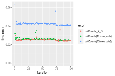
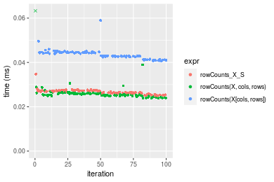Table: Benchmarking of colCounts_X_S() and rowCounts_X_S() on double+100x100 data (original and transposed). The top panel shows times in milliseconds and the bottom panel shows relative times.

	expr	min	lq	mean	median	uq	max
1	colCounts_X_S	23.562	24.5255	25.34633	25.1330	25.4070	43.858
2	rowCounts_X_S	24.849	26.1230	26.68877	26.8805	27.2565	34.776

	expr	min	lq	mean	median	uq	max
1	colCounts_X_S	1.000000	1.000000	1.000000	1.00000	1.000000	1.0000000
2	rowCounts_X_S	1.054622	1.065136	1.052964	1.06953	1.072795	0.7929226

Figure: Benchmarking of colCounts_X_S() and rowCounts_X_S() on double+100x100 data (original and transposed). Outliers are displayed as crosses. Times are in milliseconds.

1000x10 matrix

> X <- data[["1000x10"]]
> rows <- sample.int(nrow(X), size = nrow(X) * 0.7)
> cols <- sample.int(ncol(X), size = ncol(X) * 0.7)
> X_S <- X[rows, cols]
> value <- 42

> colStats <- microbenchmark(colCounts_X_S = colCounts(X_S, value = value, na.rm = FALSE), `colCounts(X, rows, cols)` = colCounts(X, 
+     value = value, na.rm = FALSE, rows = rows, cols = cols), `colCounts(X[rows, cols])` = colCounts(X[rows, 
+     cols], value = value, na.rm = FALSE), unit = "ms")

> X <- t(X)
> X_S <- t(X_S)

> rowStats <- microbenchmark(rowCounts_X_S = rowCounts(X_S, value = value, na.rm = FALSE), `rowCounts(X, cols, rows)` = rowCounts(X, 
+     value = value, na.rm = FALSE, rows = cols, cols = rows), `rowCounts(X[cols, rows])` = rowCounts(X[cols, 
+     rows], value = value, na.rm = FALSE), unit = "ms")

Table: Benchmarking of colCounts_X_S(), colCounts(X, rows, cols)() and colCounts(X[rows, cols])() on double+1000x10 data. The top panel shows times in milliseconds and the bottom panel shows relative times.

	expr	min	lq	mean	median	uq	max
1	colCounts_X_S	0.021898	0.022830	0.0233296	0.0232315	0.0234805	0.037775
2	colCounts(X, rows, cols)	0.025327	0.025928	0.0266916	0.0266655	0.0269225	0.035321
3	colCounts(X[rows, cols])	0.039135	0.039871	0.0415080	0.0411200	0.0413845	0.093472

	expr	min	lq	mean	median	uq	max
1	colCounts_X_S	1.000000	1.000000	1.000000	1.000000	1.000000	1.0000000
2	colCounts(X, rows, cols)	1.156590	1.135699	1.144109	1.147817	1.146590	0.9350364
3	colCounts(X[rows, cols])	1.787149	1.746430	1.779199	1.770010	1.762505	2.4744408

Table: Benchmarking of rowCounts_X_S(), rowCounts(X, cols, rows)() and rowCounts(X[cols, rows])() on double+1000x10 data (transposed). The top panel shows times in milliseconds and the bottom panel shows relative times.

	expr	min	lq	mean	median	uq	max
1	rowCounts_X_S	0.024659	0.0256775	0.0268400	0.026423	0.0273805	0.041143
2	rowCounts(X, cols, rows)	0.026295	0.0268980	0.0283563	0.028747	0.0290340	0.047225
3	rowCounts(X[cols, rows])	0.043929	0.0446115	0.0473452	0.047776	0.0481285	0.098369

	expr	min	lq	mean	median	uq	max
1	rowCounts_X_S	1.000000	1.000000	1.000000	1.000000	1.000000	1.000000
2	rowCounts(X, cols, rows)	1.066345	1.047532	1.056494	1.087954	1.060390	1.147826
3	rowCounts(X[cols, rows])	1.781459	1.737377	1.763981	1.808122	1.757766	2.390905

Figure: Benchmarking of colCounts_X_S(), colCounts(X, rows, cols)() and colCounts(X[rows, cols])() on double+1000x10 data as well as rowCounts_X_S(), rowCounts(X, cols, rows)() and rowCounts(X[cols, rows])() on the same data transposed. Outliers are displayed as crosses. Times are in milliseconds.

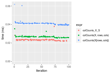
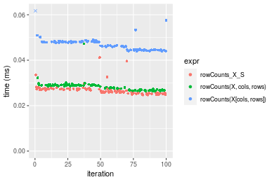Table: Benchmarking of colCounts_X_S() and rowCounts_X_S() on double+1000x10 data (original and transposed). The top panel shows times in milliseconds and the bottom panel shows relative times.

	expr	min	lq	mean	median	uq	max
1	colCounts_X_S	21.898	22.8300	23.32962	23.2315	23.4805	37.775
2	rowCounts_X_S	24.659	25.6775	26.84000	26.4230	27.3805	41.143

	expr	min	lq	mean	median	uq	max
1	colCounts_X_S	1.000000	1.000000	1.000000	1.000000	1.000000	1.00000
2	rowCounts_X_S	1.126085	1.124726	1.150469	1.137378	1.166095	1.08916

Figure: Benchmarking of colCounts_X_S() and rowCounts_X_S() on double+1000x10 data (original and transposed). Outliers are displayed as crosses. Times are in milliseconds.

10x1000 matrix

> X <- data[["10x1000"]]
> rows <- sample.int(nrow(X), size = nrow(X) * 0.7)
> cols <- sample.int(ncol(X), size = ncol(X) * 0.7)
> X_S <- X[rows, cols]
> value <- 42

> colStats <- microbenchmark(colCounts_X_S = colCounts(X_S, value = value, na.rm = FALSE), `colCounts(X, rows, cols)` = colCounts(X, 
+     value = value, na.rm = FALSE, rows = rows, cols = cols), `colCounts(X[rows, cols])` = colCounts(X[rows, 
+     cols], value = value, na.rm = FALSE), unit = "ms")

> X <- t(X)
> X_S <- t(X_S)

> rowStats <- microbenchmark(rowCounts_X_S = rowCounts(X_S, value = value, na.rm = FALSE), `rowCounts(X, cols, rows)` = rowCounts(X, 
+     value = value, na.rm = FALSE, rows = cols, cols = rows), `rowCounts(X[cols, rows])` = rowCounts(X[cols, 
+     rows], value = value, na.rm = FALSE), unit = "ms")

Table: Benchmarking of colCounts_X_S(), colCounts(X, rows, cols)() and colCounts(X[rows, cols])() on double+10x1000 data. The top panel shows times in milliseconds and the bottom panel shows relative times.

	expr	min	lq	mean	median	uq	max
1	colCounts_X_S	0.022503	0.0234300	0.0251250	0.0243615	0.0249190	0.089457
2	colCounts(X, rows, cols)	0.025854	0.0265120	0.0286491	0.0272645	0.0281910	0.078877
3	colCounts(X[rows, cols])	0.040596	0.0420115	0.0435707	0.0427890	0.0441665	0.078030

	expr	min	lq	mean	median	uq	max
1	colCounts_X_S	1.000000	1.000000	1.000000	1.000000	1.000000	1.0000000
2	colCounts(X, rows, cols)	1.148913	1.131541	1.140262	1.119163	1.131305	0.8817309
3	colCounts(X[rows, cols])	1.804026	1.793064	1.734155	1.756419	1.772403	0.8722627

Table: Benchmarking of rowCounts_X_S(), rowCounts(X, cols, rows)() and rowCounts(X[cols, rows])() on double+10x1000 data (transposed). The top panel shows times in milliseconds and the bottom panel shows relative times.

	expr	min	lq	mean	median	uq	max
1	rowCounts_X_S	0.024517	0.0258940	0.0267874	0.0268080	0.0272800	0.040653
2	rowCounts(X, cols, rows)	0.025889	0.0266410	0.0282871	0.0280125	0.0285635	0.075981
3	rowCounts(X[cols, rows])	0.041282	0.0422135	0.0439394	0.0447350	0.0450755	0.049755

	expr	min	lq	mean	median	uq	max
1	rowCounts_X_S	1.000000	1.000000	1.000000	1.000000	1.000000	1.000000
2	rowCounts(X, cols, rows)	1.055961	1.028848	1.055986	1.044931	1.047049	1.869013
3	rowCounts(X[cols, rows])	1.683811	1.630243	1.640302	1.668718	1.652328	1.223895

Figure: Benchmarking of colCounts_X_S(), colCounts(X, rows, cols)() and colCounts(X[rows, cols])() on double+10x1000 data as well as rowCounts_X_S(), rowCounts(X, cols, rows)() and rowCounts(X[cols, rows])() on the same data transposed. Outliers are displayed as crosses. Times are in milliseconds.

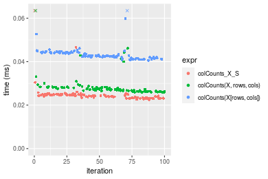
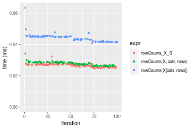Table: Benchmarking of colCounts_X_S() and rowCounts_X_S() on double+10x1000 data (original and transposed). The top panel shows times in milliseconds and the bottom panel shows relative times.

	expr	min	lq	mean	median	uq	max
1	colCounts_X_S	22.503	23.430	25.12503	24.3615	24.919	89.457
2	rowCounts_X_S	24.517	25.894	26.78740	26.8080	27.280	40.653

	expr	min	lq	mean	median	uq	max
1	colCounts_X_S	1.000000	1.000000	1.000000	1.000000	1.000000	1.0000000
2	rowCounts_X_S	1.089499	1.105164	1.066164	1.100425	1.094747	0.4544418

Figure: Benchmarking of colCounts_X_S() and rowCounts_X_S() on double+10x1000 data (original and transposed). Outliers are displayed as crosses. Times are in milliseconds.

100x1000 matrix

> X <- data[["100x1000"]]
> rows <- sample.int(nrow(X), size = nrow(X) * 0.7)
> cols <- sample.int(ncol(X), size = ncol(X) * 0.7)
> X_S <- X[rows, cols]
> value <- 42

> colStats <- microbenchmark(colCounts_X_S = colCounts(X_S, value = value, na.rm = FALSE), `colCounts(X, rows, cols)` = colCounts(X, 
+     value = value, na.rm = FALSE, rows = rows, cols = cols), `colCounts(X[rows, cols])` = colCounts(X[rows, 
+     cols], value = value, na.rm = FALSE), unit = "ms")

> X <- t(X)
> X_S <- t(X_S)

> rowStats <- microbenchmark(rowCounts_X_S = rowCounts(X_S, value = value, na.rm = FALSE), `rowCounts(X, cols, rows)` = rowCounts(X, 
+     value = value, na.rm = FALSE, rows = cols, cols = rows), `rowCounts(X[cols, rows])` = rowCounts(X[cols, 
+     rows], value = value, na.rm = FALSE), unit = "ms")

Table: Benchmarking of colCounts_X_S(), colCounts(X, rows, cols)() and colCounts(X[rows, cols])() on double+100x1000 data. The top panel shows times in milliseconds and the bottom panel shows relative times.

	expr	min	lq	mean	median	uq	max
2	colCounts(X, rows, cols)	0.105265	0.1145630	0.1307565	0.1261115	0.1394125	0.272958
1	colCounts_X_S	0.106458	0.1133215	0.1311436	0.1270160	0.1400905	0.222013
3	colCounts(X[rows, cols])	0.205337	0.2245500	0.2552749	0.2516795	0.2707955	0.342214

	expr	min	lq	mean	median	uq	max
2	colCounts(X, rows, cols)	1.000000	1.0000000	1.000000	1.000000	1.000000	1.0000000
1	colCounts_X_S	1.011333	0.9891632	1.002960	1.007172	1.004863	0.8133596
3	colCounts(X[rows, cols])	1.950667	1.9600569	1.952293	1.995690	1.942405	1.2537240

Table: Benchmarking of rowCounts_X_S(), rowCounts(X, cols, rows)() and rowCounts(X[cols, rows])() on double+100x1000 data (transposed). The top panel shows times in milliseconds and the bottom panel shows relative times.

	expr	min	lq	mean	median	uq	max
2	rowCounts(X, cols, rows)	0.118166	0.1270350	0.1429773	0.136608	0.151287	0.286464
1	rowCounts_X_S	0.127269	0.1444980	0.1596030	0.155822	0.173422	0.242767
3	rowCounts(X[cols, rows])	0.230335	0.2537255	0.2770089	0.269141	0.295137	0.364153

	expr	min	lq	mean	median	uq	max
2	rowCounts(X, cols, rows)	1.000000	1.000000	1.000000	1.000000	1.000000	1.0000000
1	rowCounts_X_S	1.077036	1.137466	1.116282	1.140651	1.146311	0.8474608
3	rowCounts(X[cols, rows])	1.949249	1.997288	1.937433	1.970170	1.950842	1.2711999

Figure: Benchmarking of colCounts_X_S(), colCounts(X, rows, cols)() and colCounts(X[rows, cols])() on double+100x1000 data as well as rowCounts_X_S(), rowCounts(X, cols, rows)() and rowCounts(X[cols, rows])() on the same data transposed. Outliers are displayed as crosses. Times are in milliseconds.

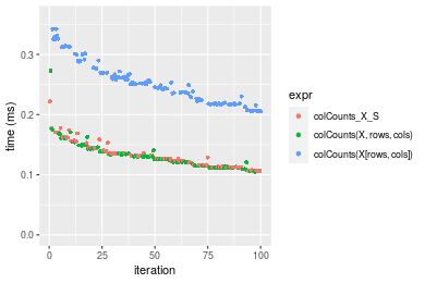
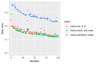Table: Benchmarking of colCounts_X_S() and rowCounts_X_S() on double+100x1000 data (original and transposed). The top panel shows times in milliseconds and the bottom panel shows relative times.

	expr	min	lq	mean	median	uq	max
1	colCounts_X_S	106.458	113.3215	131.1436	127.016	140.0905	222.013
2	rowCounts_X_S	127.269	144.4980	159.6029	155.822	173.4220	242.767

	expr	min	lq	mean	median	uq	max
1	colCounts_X_S	1.000000	1.000000	1.000000	1.00000	1.000000	1.000000
2	rowCounts_X_S	1.195485	1.275116	1.217009	1.22679	1.237928	1.093481

Figure: Benchmarking of colCounts_X_S() and rowCounts_X_S() on double+100x1000 data (original and transposed). Outliers are displayed as crosses. Times are in milliseconds.

1000x100 matrix

> X <- data[["1000x100"]]
> rows <- sample.int(nrow(X), size = nrow(X) * 0.7)
> cols <- sample.int(ncol(X), size = ncol(X) * 0.7)
> X_S <- X[rows, cols]
> value <- 42

> colStats <- microbenchmark(colCounts_X_S = colCounts(X_S, value = value, na.rm = FALSE), `colCounts(X, rows, cols)` = colCounts(X, 
+     value = value, na.rm = FALSE, rows = rows, cols = cols), `colCounts(X[rows, cols])` = colCounts(X[rows, 
+     cols], value = value, na.rm = FALSE), unit = "ms")

> X <- t(X)
> X_S <- t(X_S)

> rowStats <- microbenchmark(rowCounts_X_S = rowCounts(X_S, value = value, na.rm = FALSE), `rowCounts(X, cols, rows)` = rowCounts(X, 
+     value = value, na.rm = FALSE, rows = cols, cols = rows), `rowCounts(X[cols, rows])` = rowCounts(X[cols, 
+     rows], value = value, na.rm = FALSE), unit = "ms")

Table: Benchmarking of colCounts_X_S(), colCounts(X, rows, cols)() and colCounts(X[rows, cols])() on double+1000x100 data. The top panel shows times in milliseconds and the bottom panel shows relative times.

	expr	min	lq	mean	median	uq	max
1	colCounts_X_S	0.098470	0.112016	0.1226457	0.1197715	0.1268565	0.204858
2	colCounts(X, rows, cols)	0.103196	0.118934	0.1316289	0.1272435	0.1386230	0.220735
3	colCounts(X[rows, cols])	0.194508	0.219782	0.2492169	0.2412725	0.2593015	0.418089

	expr	min	lq	mean	median	uq	max
1	colCounts_X_S	1.000000	1.000000	1.000000	1.000000	1.000000	1.000000
2	colCounts(X, rows, cols)	1.047994	1.061759	1.073245	1.062385	1.092754	1.077503
3	colCounts(X[rows, cols])	1.975302	1.962059	2.032007	2.014440	2.044054	2.040872

Table: Benchmarking of rowCounts_X_S(), rowCounts(X, cols, rows)() and rowCounts(X[cols, rows])() on double+1000x100 data (transposed). The top panel shows times in milliseconds and the bottom panel shows relative times.

	expr	min	lq	mean	median	uq	max
2	rowCounts(X, cols, rows)	0.112588	0.1312890	0.1470693	0.1423215	0.1570235	0.330036
1	rowCounts_X_S	0.123777	0.1381475	0.1605944	0.1563945	0.1759205	0.248206
3	rowCounts(X[cols, rows])	0.219814	0.2511030	0.2845926	0.2783760	0.3158320	0.416945

	expr	min	lq	mean	median	uq	max
2	rowCounts(X, cols, rows)	1.000000	1.000000	1.000000	1.000000	1.000000	1.0000000
1	rowCounts_X_S	1.099380	1.052240	1.091964	1.098882	1.120345	0.7520574
3	rowCounts(X[cols, rows])	1.952375	1.912597	1.935092	1.955966	2.011368	1.2633319

Figure: Benchmarking of colCounts_X_S(), colCounts(X, rows, cols)() and colCounts(X[rows, cols])() on double+1000x100 data as well as rowCounts_X_S(), rowCounts(X, cols, rows)() and rowCounts(X[cols, rows])() on the same data transposed. Outliers are displayed as crosses. Times are in milliseconds.

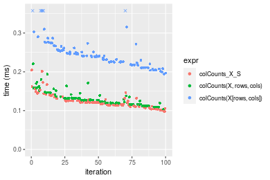
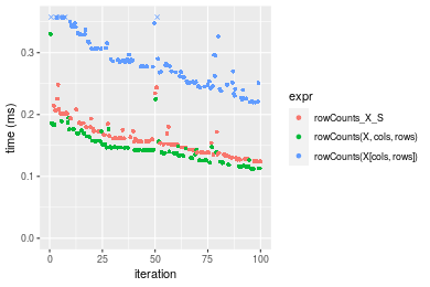Table: Benchmarking of colCounts_X_S() and rowCounts_X_S() on double+1000x100 data (original and transposed). The top panel shows times in milliseconds and the bottom panel shows relative times.

	expr	min	lq	mean	median	uq	max
1	colCounts_X_S	98.470	112.0160	122.6457	119.7715	126.8565	204.858
2	rowCounts_X_S	123.777	138.1475	160.5944	156.3945	175.9205	248.206

	expr	min	lq	mean	median	uq	max
1	colCounts_X_S	1.000000	1.000000	1.000000	1.000000	1.000000	1.0000
2	rowCounts_X_S	1.257002	1.233284	1.309417	1.305774	1.386768	1.2116

Figure: Benchmarking of colCounts_X_S() and rowCounts_X_S() on double+1000x100 data (original and transposed). Outliers are displayed as crosses. Times are in milliseconds.

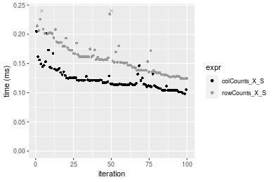
Appendix

Session information

R version 4.1.1 Patched (2021-08-10 r80727)
Platform: x86_64-pc-linux-gnu (64-bit)
Running under: Ubuntu 18.04.5 LTS

Matrix products: default
BLAS:   /home/hb/software/R-devel/R-4-1-branch/lib/R/lib/libRblas.so
LAPACK: /home/hb/software/R-devel/R-4-1-branch/lib/R/lib/libRlapack.so

locale:
 [1] LC_CTYPE=en_US.UTF-8       LC_NUMERIC=C              
 [3] LC_TIME=en_US.UTF-8        LC_COLLATE=en_US.UTF-8    
 [5] LC_MONETARY=en_US.UTF-8    LC_MESSAGES=en_US.UTF-8   
 [7] LC_PAPER=en_US.UTF-8       LC_NAME=C                 
 [9] LC_ADDRESS=C               LC_TELEPHONE=C            
[11] LC_MEASUREMENT=en_US.UTF-8 LC_IDENTIFICATION=C       

attached base packages:
[1] stats     graphics  grDevices utils     datasets  methods   base     

other attached packages:
[1] microbenchmark_1.4-7   matrixStats_0.60.1     ggplot2_3.3.5         
[4] knitr_1.33             R.devices_2.17.0       R.utils_2.10.1        
[7] R.oo_1.24.0            R.methodsS3_1.8.1-9001 history_0.0.1-9000    

loaded via a namespace (and not attached):
 [1] Biobase_2.52.0          httr_1.4.2              splines_4.1.1          
 [4] bit64_4.0.5             network_1.17.1          assertthat_0.2.1       
 [7] highr_0.9               stats4_4.1.1            blob_1.2.2             
[10] GenomeInfoDbData_1.2.6  robustbase_0.93-8       pillar_1.6.2           
[13] RSQLite_2.2.8           lattice_0.20-44         glue_1.4.2             
[16] digest_0.6.27           XVector_0.32.0          colorspace_2.0-2       
[19] Matrix_1.3-4            XML_3.99-0.7            pkgconfig_2.0.3        
[22] zlibbioc_1.38.0         genefilter_1.74.0       purrr_0.3.4            
[25] ergm_4.1.2              xtable_1.8-4            scales_1.1.1           
[28] tibble_3.1.4            annotate_1.70.0         KEGGREST_1.32.0        
[31] farver_2.1.0            generics_0.1.0          IRanges_2.26.0         
[34] ellipsis_0.3.2          cachem_1.0.6            withr_2.4.2            
[37] BiocGenerics_0.38.0     mime_0.11               survival_3.2-13        
[40] magrittr_2.0.1          crayon_1.4.1            statnet.common_4.5.0   
[43] memoise_2.0.0           laeken_0.5.1            fansi_0.5.0            
[46] R.cache_0.15.0          MASS_7.3-54             R.rsp_0.44.0           
[49] progressr_0.8.0         tools_4.1.1             lifecycle_1.0.0        
[52] S4Vectors_0.30.0        trust_0.1-8             munsell_0.5.0          
[55] tabby_0.0.1-9001        AnnotationDbi_1.54.1    Biostrings_2.60.2      
[58] compiler_4.1.1          GenomeInfoDb_1.28.1     rlang_0.4.11           
[61] grid_4.1.1              RCurl_1.98-1.4          cwhmisc_6.6            
[64] rappdirs_0.3.3          startup_0.15.0          labeling_0.4.2         
[67] bitops_1.0-7            base64enc_0.1-3         boot_1.3-28            
[70] gtable_0.3.0            DBI_1.1.1               markdown_1.1           
[73] R6_2.5.1                lpSolveAPI_5.5.2.0-17.7 rle_0.9.2              
[76] dplyr_1.0.7             fastmap_1.1.0           bit_4.0.4              
[79] utf8_1.2.2              parallel_4.1.1          Rcpp_1.0.7             
[82] vctrs_0.3.8             png_0.1-7               DEoptimR_1.0-9         
[85] tidyselect_1.1.1        xfun_0.25               coda_0.19-4            

Total processing time was 34.05 secs.

Reproducibility

To reproduce this report, do:

html <- matrixStats:::benchmark('colRowCounts_subset')