matrixStats.benchmarks
madDiff() benchmarks
This report benchmark the performance of madDiff() against alternative methods.
Alternative methods
- N/A
Data type “integer”
Data
> rvector <- function(n, mode = c("logical", "double", "integer"), range = c(-100, +100), na_prob = 0) {
+     mode <- match.arg(mode)
+     if (mode == "logical") {
+         x <- sample(c(FALSE, TRUE), size = n, replace = TRUE)
+     }     else {
+         x <- runif(n, min = range[1], max = range[2])
+     }
+     storage.mode(x) <- mode
+     if (na_prob > 0)
+         x[sample(n, size = na_prob * n)] <- NA
+     x
+ }
> rvectors <- function(scale = 10, seed = 1, ...) {
+     set.seed(seed)
+     data <- list()
+     data[[1]] <- rvector(n = scale * 100, ...)
+     data[[2]] <- rvector(n = scale * 1000, ...)
+     data[[3]] <- rvector(n = scale * 10000, ...)
+     data[[4]] <- rvector(n = scale * 1e+05, ...)
+     data[[5]] <- rvector(n = scale * 1e+06, ...)
+     names(data) <- sprintf("n = %d", sapply(data, FUN = length))
+     data
+ }
> data <- rvectors(mode = mode)
> data <- data[1:4]
Results
n = 1000 vector
All elements
> x <- data[["n = 1000"]]
> stats <- microbenchmark(madDiff = madDiff(x), mad = mad(x), diff = diff(x), unit = "ms")
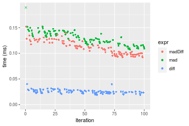
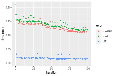
Table: Benchmarking of madDiff(), mad() and diff() on integer+n = 1000 data. The top panel shows times in milliseconds and the bottom panel shows relative times.
| expr | min | lq | mean | median | uq | max | |
|---|---|---|---|---|---|---|---|
| 3 | diff | 0.018767 | 0.0231650 | 0.0253068 | 0.0248335 | 0.0273700 | 0.040044 |
| 1 | madDiff | 0.092016 | 0.0986185 | 0.1110708 | 0.1105605 | 0.1231885 | 0.151665 |
| 2 | mad | 0.107037 | 0.1189425 | 0.1308682 | 0.1291255 | 0.1400280 | 0.275417 |
| expr | min | lq | mean | median | uq | max | |
|---|---|---|---|---|---|---|---|
| 3 | diff | 1.000000 | 1.000000 | 1.000000 | 1.000000 | 1.000000 | 1.000000 |
| 1 | madDiff | 4.903074 | 4.257220 | 4.388962 | 4.452071 | 4.500859 | 3.787459 |
| 2 | mad | 5.703469 | 5.134578 | 5.171258 | 5.199650 | 5.116112 | 6.877859 |
Figure: Benchmarking of madDiff(), mad() and diff() on integer+n = 1000 data. Outliers are displayed as crosses. Times are in milliseconds.
n = 10000 vector
All elements
> x <- data[["n = 10000"]]
> stats <- microbenchmark(madDiff = madDiff(x), mad = mad(x), diff = diff(x), unit = "ms")
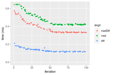
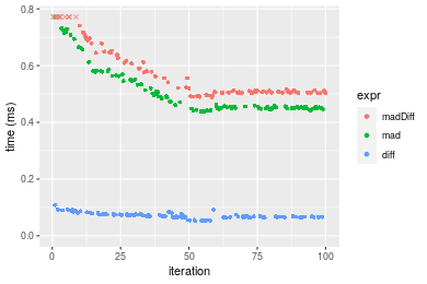
Table: Benchmarking of madDiff(), mad() and diff() on integer+n = 10000 data. The top panel shows times in milliseconds and the bottom panel shows relative times.
| expr | min | lq | mean | median | uq | max | |
|---|---|---|---|---|---|---|---|
| 3 | diff | 0.112008 | 0.1190410 | 0.1346192 | 0.126125 | 0.1444330 | 0.211025 |
| 1 | madDiff | 0.327303 | 0.3328905 | 0.3857618 | 0.338831 | 0.4275240 | 0.655837 |
| 2 | mad | 0.411850 | 0.4206475 | 0.4807517 | 0.431365 | 0.5258605 | 0.746280 |
| expr | min | lq | mean | median | uq | max | |
|---|---|---|---|---|---|---|---|
| 3 | diff | 1.000000 | 1.000000 | 1.000000 | 1.000000 | 1.000000 | 1.000000 |
| 1 | madDiff | 2.922140 | 2.796436 | 2.865578 | 2.686470 | 2.960016 | 3.107864 |
| 2 | mad | 3.676969 | 3.533635 | 3.571197 | 3.420139 | 3.640861 | 3.536453 |
Figure: Benchmarking of madDiff(), mad() and diff() on integer+n = 10000 data. Outliers are displayed as crosses. Times are in milliseconds.
n = 100000 vector
All elements
> x <- data[["n = 100000"]]
> stats <- microbenchmark(madDiff = madDiff(x), mad = mad(x), diff = diff(x), unit = "ms")
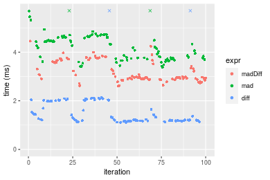
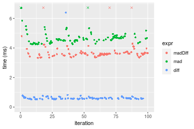
Table: Benchmarking of madDiff(), mad() and diff() on integer+n = 100000 data. The top panel shows times in milliseconds and the bottom panel shows relative times.
| expr | min | lq | mean | median | uq | max | |
|---|---|---|---|---|---|---|---|
| 3 | diff | 1.109217 | 1.178817 | 1.601809 | 1.249338 | 1.996576 | 8.068402 |
| 1 | madDiff | 2.608344 | 2.893647 | 3.187560 | 2.967735 | 3.629499 | 4.456352 |
| 2 | mad | 3.370880 | 3.716534 | 4.424291 | 4.195974 | 4.606384 | 17.683648 |
| expr | min | lq | mean | median | uq | max | |
|---|---|---|---|---|---|---|---|
| 3 | diff | 1.000000 | 1.000000 | 1.000000 | 1.000000 | 1.000000 | 1.0000000 |
| 1 | madDiff | 2.351518 | 2.454704 | 1.989975 | 2.375445 | 1.817862 | 0.5523215 |
| 2 | mad | 3.038972 | 3.152766 | 2.762058 | 3.358557 | 2.307143 | 2.1917163 |
Figure: Benchmarking of madDiff(), mad() and diff() on integer+n = 100000 data. Outliers are displayed as crosses. Times are in milliseconds.
n = 1000000 vector
All elements
> x <- data[["n = 1000000"]]
> stats <- microbenchmark(madDiff = madDiff(x), mad = mad(x), diff = diff(x), unit = "ms")
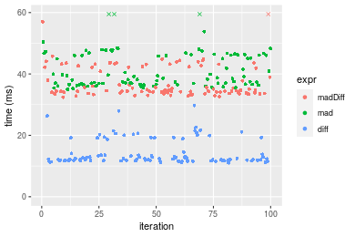
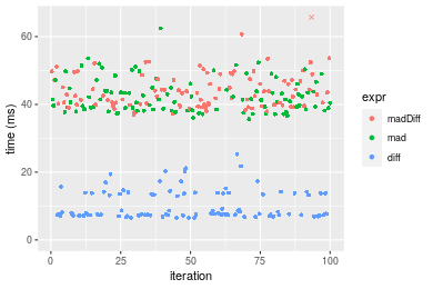
Table: Benchmarking of madDiff(), mad() and diff() on integer+n = 1000000 data. The top panel shows times in milliseconds and the bottom panel shows relative times.
| expr | min | lq | mean | median | uq | max | |
|---|---|---|---|---|---|---|---|
| 3 | diff | 11.04763 | 11.81992 | 14.44155 | 12.34955 | 16.62525 | 29.71610 |
| 1 | madDiff | 32.44946 | 33.97319 | 41.23050 | 34.63759 | 42.31104 | 444.32295 |
| 2 | mad | 35.01356 | 36.80087 | 41.85479 | 38.95332 | 46.30287 | 81.67478 |
| expr | min | lq | mean | median | uq | max | |
|---|---|---|---|---|---|---|---|
| 3 | diff | 1.000000 | 1.000000 | 1.000000 | 1.000000 | 1.000000 | 1.000000 |
| 1 | madDiff | 2.937234 | 2.874232 | 2.854992 | 2.804765 | 2.544986 | 14.952261 |
| 2 | mad | 3.169329 | 3.113462 | 2.898221 | 3.154229 | 2.785093 | 2.748502 |
Figure: Benchmarking of madDiff(), mad() and diff() on integer+n = 1000000 data. Outliers are displayed as crosses. Times are in milliseconds.
Data type “double”
Data
> rvector <- function(n, mode = c("logical", "double", "integer"), range = c(-100, +100), na_prob = 0) {
+     mode <- match.arg(mode)
+     if (mode == "logical") {
+         x <- sample(c(FALSE, TRUE), size = n, replace = TRUE)
+     }     else {
+         x <- runif(n, min = range[1], max = range[2])
+     }
+     storage.mode(x) <- mode
+     if (na_prob > 0)
+         x[sample(n, size = na_prob * n)] <- NA
+     x
+ }
> rvectors <- function(scale = 10, seed = 1, ...) {
+     set.seed(seed)
+     data <- list()
+     data[[1]] <- rvector(n = scale * 100, ...)
+     data[[2]] <- rvector(n = scale * 1000, ...)
+     data[[3]] <- rvector(n = scale * 10000, ...)
+     data[[4]] <- rvector(n = scale * 1e+05, ...)
+     data[[5]] <- rvector(n = scale * 1e+06, ...)
+     names(data) <- sprintf("n = %d", sapply(data, FUN = length))
+     data
+ }
> data <- rvectors(mode = mode)
> data <- data[1:4]
Results
n = 1000 vector
All elements
> x <- data[["n = 1000"]]
> stats <- microbenchmark(madDiff = madDiff(x), mad = mad(x), diff = diff(x), unit = "ms")
Table: Benchmarking of madDiff(), mad() and diff() on double+n = 1000 data. The top panel shows times in milliseconds and the bottom panel shows relative times.
| expr | min | lq | mean | median | uq | max | |
|---|---|---|---|---|---|---|---|
| 3 | diff | 0.013108 | 0.0156105 | 0.0175863 | 0.016575 | 0.018627 | 0.035798 |
| 1 | madDiff | 0.110005 | 0.1140300 | 0.1274836 | 0.124992 | 0.139961 | 0.174583 |
| 2 | mad | 0.117293 | 0.1291395 | 0.1404472 | 0.141437 | 0.148812 | 0.293020 |
| expr | min | lq | mean | median | uq | max | |
|---|---|---|---|---|---|---|---|
| 3 | diff | 1.000000 | 1.000000 | 1.000000 | 1.000000 | 1.000000 | 1.000000 |
| 1 | madDiff | 8.392203 | 7.304699 | 7.249051 | 7.540996 | 7.513878 | 4.876893 |
| 2 | mad | 8.948200 | 8.272605 | 7.986194 | 8.533152 | 7.989048 | 8.185374 |
Figure: Benchmarking of madDiff(), mad() and diff() on double+n = 1000 data. Outliers are displayed as crosses. Times are in milliseconds.
n = 10000 vector
All elements
> x <- data[["n = 10000"]]
> stats <- microbenchmark(madDiff = madDiff(x), mad = mad(x), diff = diff(x), unit = "ms")
Table: Benchmarking of madDiff(), mad() and diff() on double+n = 10000 data. The top panel shows times in milliseconds and the bottom panel shows relative times.
| expr | min | lq | mean | median | uq | max | |
|---|---|---|---|---|---|---|---|
| 3 | diff | 0.052420 | 0.0657780 | 0.0711756 | 0.0684290 | 0.0757170 | 0.108527 |
| 2 | mad | 0.436525 | 0.4495135 | 0.5078273 | 0.4580255 | 0.5511330 | 0.792393 |
| 1 | madDiff | 0.488370 | 0.5050310 | 0.5750690 | 0.5110170 | 0.6329265 | 0.945029 |
| expr | min | lq | mean | median | uq | max | |
|---|---|---|---|---|---|---|---|
| 3 | diff | 1.000000 | 1.000000 | 1.000000 | 1.000000 | 1.000000 | 1.000000 |
| 2 | mad | 8.327451 | 6.833797 | 7.134849 | 6.693441 | 7.278854 | 7.301344 |
| 1 | madDiff | 9.316482 | 7.677810 | 8.079578 | 7.467843 | 8.359107 | 8.707778 |
Figure: Benchmarking of madDiff(), mad() and diff() on double+n = 10000 data. Outliers are displayed as crosses. Times are in milliseconds.
n = 100000 vector
All elements
> x <- data[["n = 100000"]]
> stats <- microbenchmark(madDiff = madDiff(x), mad = mad(x), diff = diff(x), unit = "ms")
Table: Benchmarking of madDiff(), mad() and diff() on double+n = 100000 data. The top panel shows times in milliseconds and the bottom panel shows relative times.
| expr | min | lq | mean | median | uq | max | |
|---|---|---|---|---|---|---|---|
| 3 | diff | 0.517747 | 0.5573075 | 0.6635397 | 0.584073 | 0.6394385 | 6.394521 |
| 1 | madDiff | 3.331675 | 3.5211060 | 3.8442516 | 3.611360 | 3.7046145 | 10.335326 |
| 2 | mad | 4.246693 | 4.4425925 | 4.7458903 | 4.604933 | 4.7732830 | 10.507083 |
| expr | min | lq | mean | median | uq | max | |
|---|---|---|---|---|---|---|---|
| 3 | diff | 1.000000 | 1.000000 | 1.000000 | 1.000000 | 1.000000 | 1.000000 |
| 1 | madDiff | 6.434948 | 6.318067 | 5.793552 | 6.183064 | 5.793543 | 1.616278 |
| 2 | mad | 8.202255 | 7.971528 | 7.152384 | 7.884175 | 7.464804 | 1.643138 |
Figure: Benchmarking of madDiff(), mad() and diff() on double+n = 100000 data. Outliers are displayed as crosses. Times are in milliseconds.
n = 1000000 vector
All elements
> x <- data[["n = 1000000"]]
> stats <- microbenchmark(madDiff = madDiff(x), mad = mad(x), diff = diff(x), unit = "ms")
Table: Benchmarking of madDiff(), mad() and diff() on double+n = 1000000 data. The top panel shows times in milliseconds and the bottom panel shows relative times.
| expr | min | lq | mean | median | uq | max | |
|---|---|---|---|---|---|---|---|
| 3 | diff | 6.467412 | 7.319129 | 10.30967 | 7.688428 | 13.78460 | 25.29299 |
| 2 | mad | 35.638038 | 38.530104 | 42.55627 | 41.443557 | 44.88876 | 62.42188 |
| 1 | madDiff | 36.931001 | 39.894058 | 47.82656 | 42.899650 | 47.32208 | 438.69708 |
| expr | min | lq | mean | median | uq | max | |
|---|---|---|---|---|---|---|---|
| 3 | diff | 1.000000 | 1.000000 | 1.000000 | 1.000000 | 1.000000 | 1.000000 |
| 2 | mad | 5.510402 | 5.264302 | 4.127803 | 5.390381 | 3.256442 | 2.467952 |
| 1 | madDiff | 5.710321 | 5.450657 | 4.639003 | 5.579768 | 3.432966 | 17.344613 |
Figure: Benchmarking of madDiff(), mad() and diff() on double+n = 1000000 data. Outliers are displayed as crosses. Times are in milliseconds.
Appendix
Session information
R version 4.1.1 Patched (2021-08-10 r80727)
Platform: x86_64-pc-linux-gnu (64-bit)
Running under: Ubuntu 18.04.5 LTS

Matrix products: default
BLAS:   /home/hb/software/R-devel/R-4-1-branch/lib/R/lib/libRblas.so
LAPACK: /home/hb/software/R-devel/R-4-1-branch/lib/R/lib/libRlapack.so

locale:
 [1] LC_CTYPE=en_US.UTF-8       LC_NUMERIC=C
 [3] LC_TIME=en_US.UTF-8        LC_COLLATE=en_US.UTF-8
 [5] LC_MONETARY=en_US.UTF-8    LC_MESSAGES=en_US.UTF-8
 [7] LC_PAPER=en_US.UTF-8       LC_NAME=C
 [9] LC_ADDRESS=C               LC_TELEPHONE=C
[11] LC_MEASUREMENT=en_US.UTF-8 LC_IDENTIFICATION=C

attached base packages:
[1] stats     graphics  grDevices utils     datasets  methods   base

other attached packages:
[1] microbenchmark_1.4-7   matrixStats_0.60.0     ggplot2_3.3.5
[4] knitr_1.33             R.devices_2.17.0       R.utils_2.10.1
[7] R.oo_1.24.0            R.methodsS3_1.8.1-9001 history_0.0.1-9000

loaded via a namespace (and not attached):
 [1] Biobase_2.52.0          httr_1.4.2              splines_4.1.1
 [4] bit64_4.0.5             network_1.17.1          assertthat_0.2.1
 [7] highr_0.9               stats4_4.1.1            blob_1.2.2
[10] GenomeInfoDbData_1.2.6  robustbase_0.93-8       pillar_1.6.2
[13] RSQLite_2.2.8           lattice_0.20-44         glue_1.4.2
[16] digest_0.6.27           XVector_0.32.0          colorspace_2.0-2
[19] Matrix_1.3-4            XML_3.99-0.7            pkgconfig_2.0.3
[22] zlibbioc_1.38.0         genefilter_1.74.0       purrr_0.3.4
[25] ergm_4.1.2              xtable_1.8-4            scales_1.1.1
[28] tibble_3.1.4            annotate_1.70.0         KEGGREST_1.32.0
[31] farver_2.1.0            generics_0.1.0          IRanges_2.26.0
[34] ellipsis_0.3.2          cachem_1.0.6            withr_2.4.2
[37] BiocGenerics_0.38.0     mime_0.11               survival_3.2-13
[40] magrittr_2.0.1          crayon_1.4.1            statnet.common_4.5.0
[43] memoise_2.0.0           laeken_0.5.1            fansi_0.5.0
[46] R.cache_0.15.0          MASS_7.3-54             R.rsp_0.44.0
[49] progressr_0.8.0         tools_4.1.1             lifecycle_1.0.0
[52] S4Vectors_0.30.0        trust_0.1-8             munsell_0.5.0
[55] tabby_0.0.1-9001        AnnotationDbi_1.54.1    Biostrings_2.60.2
[58] compiler_4.1.1          GenomeInfoDb_1.28.1     rlang_0.4.11
[61] grid_4.1.1              RCurl_1.98-1.4          cwhmisc_6.6
[64] rstudioapi_0.13         rappdirs_0.3.3          startup_0.15.0-9000
[67] labeling_0.4.2          bitops_1.0-7            base64enc_0.1-3
[70] boot_1.3-28             gtable_0.3.0            DBI_1.1.1
[73] markdown_1.1            R6_2.5.1                lpSolveAPI_5.5.2.0-17.7
[76] rle_0.9.2               dplyr_1.0.7             fastmap_1.1.0
[79] bit_4.0.4               utf8_1.2.2              parallel_4.1.1
[82] Rcpp_1.0.7              vctrs_0.3.8             png_0.1-7
[85] DEoptimR_1.0-9          tidyselect_1.1.1        xfun_0.25
[88] coda_0.19-4
Total processing time was 30.23 secs.
Reproducibility
To reproduce this report, do:
html <- matrixStats:::benchmark('madDiff')
Copyright Henrik Bengtsson. Last updated on 2021-08-25 22:40:59 (+0200 UTC). Powered by RSP.