matrixStats.benchmarks
count() benchmarks on subsetted computation
This report benchmark the performance of count() on subsetted computation.
Data type “integer”
Data
> rvector <- function(n, mode = c("logical", "double", "integer"), range = c(-100, +100), na_prob = 0) {
+     mode <- match.arg(mode)
+     if (mode == "logical") {
+         x <- sample(c(FALSE, TRUE), size = n, replace = TRUE)
+     }     else {
+         x <- runif(n, min = range[1], max = range[2])
+     }
+     storage.mode(x) <- mode
+     if (na_prob > 0)
+         x[sample(n, size = na_prob * n)] <- NA
+     x
+ }
> rvectors <- function(scale = 10, seed = 1, ...) {
+     set.seed(seed)
+     data <- list()
+     data[[1]] <- rvector(n = scale * 100, ...)
+     data[[2]] <- rvector(n = scale * 1000, ...)
+     data[[3]] <- rvector(n = scale * 10000, ...)
+     data[[4]] <- rvector(n = scale * 1e+05, ...)
+     data[[5]] <- rvector(n = scale * 1e+06, ...)
+     names(data) <- sprintf("n = %d", sapply(data, FUN = length))
+     data
+ }
> data <- rvectors(mode = mode)
Results
n = 1000 vector
> x <- data[["n = 1000"]]
> idxs <- sample.int(length(x), size = length(x) * 0.7)
> x_S <- x[idxs]
> gc()
           used  (Mb) gc trigger  (Mb) max used  (Mb)
Ncells  5340542 285.3    7916910 422.9  7916910 422.9
Vcells 16210635 123.7   33191153 253.3 53339345 407.0
> stats <- microbenchmark(count_x_S = count(x_S, value), `count(x, idxs)` = count(x, idxs = idxs, value),
+     `count(x[idxs])` = count(x[idxs], value), unit = "ms")
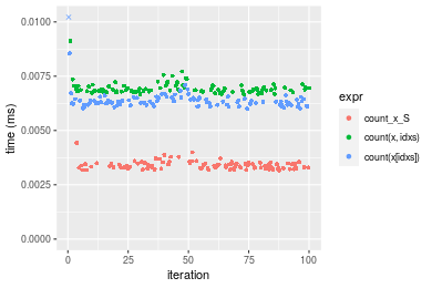
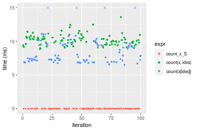
Table: Benchmarking of count_x_S(), count(x, idxs)() and count(x[idxs])() on integer+n = 1000 data. The top panel shows times in milliseconds and the bottom panel shows relative times.
| expr | min | lq | mean | median | uq | max | |
|---|---|---|---|---|---|---|---|
| 1 | count_x_S | 0.003165 | 0.0032770 | 0.0034036 | 0.0033775 | 0.0034830 | 0.004430 |
| 3 | count(x[idxs]) | 0.006003 | 0.0061900 | 0.0083801 | 0.0063200 | 0.0064515 | 0.208297 |
| 2 | count(x, idxs) | 0.006669 | 0.0068015 | 0.0069492 | 0.0068695 | 0.0070325 | 0.009120 |
| expr | min | lq | mean | median | uq | max | |
|---|---|---|---|---|---|---|---|
| 1 | count_x_S | 1.000000 | 1.000000 | 1.000000 | 1.000000 | 1.000000 | 1.000000 |
| 3 | count(x[idxs]) | 1.896683 | 1.888923 | 2.462111 | 1.871206 | 1.852283 | 47.019639 |
| 2 | count(x, idxs) | 2.107109 | 2.075526 | 2.041711 | 2.033901 | 2.019093 | 2.058691 |
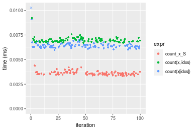
Figure: Benchmarking of count_x_S(), count(x, idxs)() and count(x[idxs])() on integer+n = 1000 data. Outliers are displayed as crosses. Times are in milliseconds.
n = 10000 vector
> x <- data[["n = 10000"]]
> idxs <- sample.int(length(x), size = length(x) * 0.7)
> x_S <- x[idxs]
> gc()
           used  (Mb) gc trigger  (Mb) max used  (Mb)
Ncells  5337927 285.1    7916910 422.9  7916910 422.9
Vcells 15878804 121.2   33191153 253.3 53339345 407.0
> stats <- microbenchmark(count_x_S = count(x_S, value), `count(x, idxs)` = count(x, idxs = idxs, value),
+     `count(x[idxs])` = count(x[idxs], value), unit = "ms")
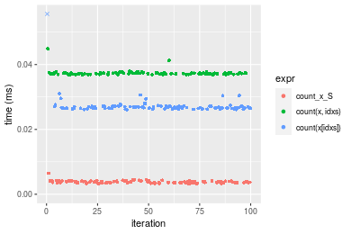
Table: Benchmarking of count_x_S(), count(x, idxs)() and count(x[idxs])() on integer+n = 10000 data. The top panel shows times in milliseconds and the bottom panel shows relative times.
| expr | min | lq | mean | median | uq | max | |
|---|---|---|---|---|---|---|---|
| 1 | count_x_S | 0.003288 | 0.003550 | 0.0038011 | 0.0037305 | 0.0040240 | 0.006466 |
| 3 | count(x[idxs]) | 0.026106 | 0.026514 | 0.0273560 | 0.0268175 | 0.0271175 | 0.063253 |
| 2 | count(x, idxs) | 0.036846 | 0.037067 | 0.0373741 | 0.0372410 | 0.0374300 | 0.044914 |
| expr | min | lq | mean | median | uq | max | |
|---|---|---|---|---|---|---|---|
| 1 | count_x_S | 1.000000 | 1.000000 | 1.000000 | 1.000000 | 1.000000 | 1.00000 |
| 3 | count(x[idxs]) | 7.939781 | 7.468732 | 7.196872 | 7.188715 | 6.738941 | 9.78240 |
| 2 | count(x, idxs) | 11.206204 | 10.441408 | 9.832472 | 9.982844 | 9.301690 | 6.94618 |
Figure: Benchmarking of count_x_S(), count(x, idxs)() and count(x[idxs])() on integer+n = 10000 data. Outliers are displayed as crosses. Times are in milliseconds.
n = 100000 vector
> x <- data[["n = 100000"]]
> idxs <- sample.int(length(x), size = length(x) * 0.7)
> x_S <- x[idxs]
> gc()
           used  (Mb) gc trigger  (Mb) max used  (Mb)
Ncells  5337999 285.1    7916910 422.9  7916910 422.9
Vcells 15942364 121.7   33191153 253.3 53339345 407.0
> stats <- microbenchmark(count_x_S = count(x_S, value), `count(x, idxs)` = count(x, idxs = idxs, value),
+     `count(x[idxs])` = count(x[idxs], value), unit = "ms")
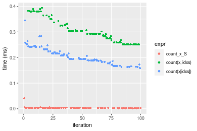
Table: Benchmarking of count_x_S(), count(x, idxs)() and count(x[idxs])() on integer+n = 100000 data. The top panel shows times in milliseconds and the bottom panel shows relative times.
| expr | min | lq | mean | median | uq | max | |
|---|---|---|---|---|---|---|---|
| 1 | count_x_S | 0.002166 | 0.002836 | 0.0036747 | 0.0032695 | 0.0036805 | 0.040622 |
| 3 | count(x[idxs]) | 0.158212 | 0.183114 | 0.2053036 | 0.1953910 | 0.2246385 | 0.344744 |
| 2 | count(x, idxs) | 0.250821 | 0.267656 | 0.3021490 | 0.2930675 | 0.3256455 | 0.394210 |
| expr | min | lq | mean | median | uq | max | |
|---|---|---|---|---|---|---|---|
| 1 | count_x_S | 1.0000 | 1.0000 | 1.00000 | 1.00000 | 1.00000 | 1.000000 |
| 3 | count(x[idxs]) | 73.0434 | 64.5677 | 55.86933 | 59.76174 | 61.03478 | 8.486633 |
| 2 | count(x, idxs) | 115.7992 | 94.3780 | 82.22391 | 89.63679 | 88.47860 | 9.704347 |
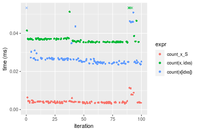
Figure: Benchmarking of count_x_S(), count(x, idxs)() and count(x[idxs])() on integer+n = 100000 data. Outliers are displayed as crosses. Times are in milliseconds.
n = 1000000 vector
> x <- data[["n = 1000000"]]
> idxs <- sample.int(length(x), size = length(x) * 0.7)
> x_S <- x[idxs]
> gc()
           used  (Mb) gc trigger  (Mb) max used  (Mb)
Ncells  5338071 285.1    7916910 422.9  7916910 422.9
Vcells 16572413 126.5   33191153 253.3 53339345 407.0
> stats <- microbenchmark(count_x_S = count(x_S, value), `count(x, idxs)` = count(x, idxs = idxs, value),
+     `count(x[idxs])` = count(x[idxs], value), unit = "ms")
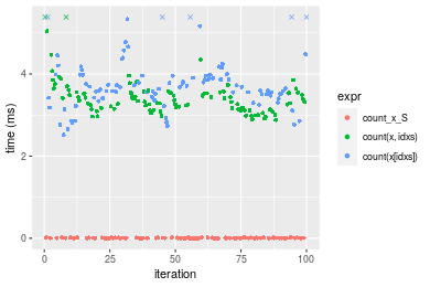
Table: Benchmarking of count_x_S(), count(x, idxs)() and count(x[idxs])() on integer+n = 1000000 data. The top panel shows times in milliseconds and the bottom panel shows relative times.
| expr | min | lq | mean | median | uq | max | |
|---|---|---|---|---|---|---|---|
| 1 | count_x_S | 0.002164 | 0.002808 | 0.0070946 | 0.0052395 | 0.011412 | 0.021826 |
| 2 | count(x, idxs) | 2.882016 | 3.146648 | 3.4423735 | 3.3550120 | 3.551007 | 6.371150 |
| 3 | count(x[idxs]) | 2.515649 | 3.430789 | 3.9598751 | 3.6643235 | 3.978525 | 15.244591 |
| expr | min | lq | mean | median | uq | max | |
|---|---|---|---|---|---|---|---|
| 1 | count_x_S | 1.0 | 1.000 | 1.0000 | 1.0000 | 1.0000 | 1.0000 |
| 2 | count(x, idxs) | 1331.8 | 1120.601 | 485.2124 | 640.3306 | 311.1643 | 291.9064 |
| 3 | count(x[idxs]) | 1162.5 | 1221.791 | 558.1558 | 699.3651 | 348.6264 | 698.4601 |
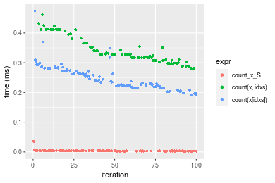
Figure: Benchmarking of count_x_S(), count(x, idxs)() and count(x[idxs])() on integer+n = 1000000 data. Outliers are displayed as crosses. Times are in milliseconds.
n = 10000000 vector
> x <- data[["n = 10000000"]]
> idxs <- sample.int(length(x), size = length(x) * 0.7)
> x_S <- x[idxs]
> gc()
           used  (Mb) gc trigger  (Mb) max used  (Mb)
Ncells  5338143 285.1    7916910 422.9  7916910 422.9
Vcells 22872461 174.6   39909383 304.5 53339345 407.0
> stats <- microbenchmark(count_x_S = count(x_S, value), `count(x, idxs)` = count(x, idxs = idxs, value),
+     `count(x[idxs])` = count(x[idxs], value), unit = "ms")
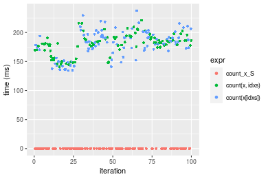
Table: Benchmarking of count_x_S(), count(x, idxs)() and count(x[idxs])() on integer+n = 10000000 data. The top panel shows times in milliseconds and the bottom panel shows relative times.
| expr | min | lq | mean | median | uq | max | |
|---|---|---|---|---|---|---|---|
| 1 | count_x_S | 0.004851 | 0.0108875 | 0.0291995 | 0.0147685 | 0.05003 | 0.096594 |
| 3 | count(x[idxs]) | 112.695468 | 144.0791635 | 151.8691124 | 151.5446780 | 161.92704 | 185.375112 |
| 2 | count(x, idxs) | 143.218317 | 171.7195710 | 178.0571528 | 178.0768070 | 186.00374 | 202.085918 |
| expr | min | lq | mean | median | uq | max | |
|---|---|---|---|---|---|---|---|
| 1 | count_x_S | 1.00 | 1.00 | 1.000 | 1.00 | 1.000 | 1.000 |
| 3 | count(x[idxs]) | 23231.39 | 13233.45 | 5201.084 | 10261.35 | 3236.599 | 1919.116 |
| 2 | count(x, idxs) | 29523.46 | 15772.18 | 6097.950 | 12057.88 | 3717.844 | 2092.117 |
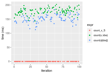
Figure: Benchmarking of count_x_S(), count(x, idxs)() and count(x[idxs])() on integer+n = 10000000 data. Outliers are displayed as crosses. Times are in milliseconds.
Data type “double”
Data
> rvector <- function(n, mode = c("logical", "double", "integer"), range = c(-100, +100), na_prob = 0) {
+     mode <- match.arg(mode)
+     if (mode == "logical") {
+         x <- sample(c(FALSE, TRUE), size = n, replace = TRUE)
+     }     else {
+         x <- runif(n, min = range[1], max = range[2])
+     }
+     storage.mode(x) <- mode
+     if (na_prob > 0)
+         x[sample(n, size = na_prob * n)] <- NA
+     x
+ }
> rvectors <- function(scale = 10, seed = 1, ...) {
+     set.seed(seed)
+     data <- list()
+     data[[1]] <- rvector(n = scale * 100, ...)
+     data[[2]] <- rvector(n = scale * 1000, ...)
+     data[[3]] <- rvector(n = scale * 10000, ...)
+     data[[4]] <- rvector(n = scale * 1e+05, ...)
+     data[[5]] <- rvector(n = scale * 1e+06, ...)
+     names(data) <- sprintf("n = %d", sapply(data, FUN = length))
+     data
+ }
> data <- rvectors(mode = mode)
Results
n = 1000 vector
> x <- data[["n = 1000"]]
> idxs <- sample.int(length(x), size = length(x) * 0.7)
> x_S <- x[idxs]
> gc()
           used  (Mb) gc trigger  (Mb) max used  (Mb)
Ncells  5338218 285.1    7916910 422.9  7916910 422.9
Vcells 21429654 163.5   39909383 304.5 53339345 407.0
> stats <- microbenchmark(count_x_S = count(x_S, value), `count(x, idxs)` = count(x, idxs = idxs, value),
+     `count(x[idxs])` = count(x[idxs], value), unit = "ms")
Table: Benchmarking of count_x_S(), count(x, idxs)() and count(x[idxs])() on double+n = 1000 data. The top panel shows times in milliseconds and the bottom panel shows relative times.
| expr | min | lq | mean | median | uq | max | |
|---|---|---|---|---|---|---|---|
| 1 | count_x_S | 0.003317 | 0.0034820 | 0.0036153 | 0.0035745 | 0.003704 | 0.004397 |
| 3 | count(x[idxs]) | 0.005992 | 0.0062655 | 0.0067630 | 0.0064005 | 0.006526 | 0.038887 |
| 2 | count(x, idxs) | 0.006709 | 0.0068305 | 0.0069903 | 0.0069360 | 0.007085 | 0.009212 |
| expr | min | lq | mean | median | uq | max | |
|---|---|---|---|---|---|---|---|
| 1 | count_x_S | 1.000000 | 1.000000 | 1.000000 | 1.000000 | 1.000000 | 1.000000 |
| 3 | count(x[idxs]) | 1.806452 | 1.799397 | 1.870666 | 1.790600 | 1.761879 | 8.843984 |
| 2 | count(x, idxs) | 2.022611 | 1.961660 | 1.933532 | 1.940411 | 1.912797 | 2.095065 |
Figure: Benchmarking of count_x_S(), count(x, idxs)() and count(x[idxs])() on double+n = 1000 data. Outliers are displayed as crosses. Times are in milliseconds.
n = 10000 vector
> x <- data[["n = 10000"]]
> idxs <- sample.int(length(x), size = length(x) * 0.7)
> x_S <- x[idxs]
> gc()
           used  (Mb) gc trigger  (Mb) max used  (Mb)
Ncells  5338287 285.1    7916910 422.9  7916910 422.9
Vcells 21439146 163.6   39909383 304.5 53339345 407.0
> stats <- microbenchmark(count_x_S = count(x_S, value), `count(x, idxs)` = count(x, idxs = idxs, value),
+     `count(x[idxs])` = count(x[idxs], value), unit = "ms")
Table: Benchmarking of count_x_S(), count(x, idxs)() and count(x[idxs])() on double+n = 10000 data. The top panel shows times in milliseconds and the bottom panel shows relative times.
| expr | min | lq | mean | median | uq | max | |
|---|---|---|---|---|---|---|---|
| 1 | count_x_S | 0.003151 | 0.0035635 | 0.0041511 | 0.0038425 | 0.0041575 | 0.011320 |
| 3 | count(x[idxs]) | 0.023584 | 0.0247065 | 0.0274833 | 0.0257360 | 0.0267605 | 0.075453 |
| 2 | count(x, idxs) | 0.035118 | 0.0354355 | 0.0376289 | 0.0358800 | 0.0370940 | 0.068346 |
| expr | min | lq | mean | median | uq | max | |
|---|---|---|---|---|---|---|---|
| 1 | count_x_S | 1.000000 | 1.000000 | 1.000000 | 1.000000 | 1.000000 | 1.000000 |
| 3 | count(x[idxs]) | 7.484608 | 6.933212 | 6.620754 | 6.697723 | 6.436681 | 6.665459 |
| 2 | count(x, idxs) | 11.145033 | 9.944016 | 9.064855 | 9.337671 | 8.922189 | 6.037632 |
Figure: Benchmarking of count_x_S(), count(x, idxs)() and count(x[idxs])() on double+n = 10000 data. Outliers are displayed as crosses. Times are in milliseconds.
n = 100000 vector
> x <- data[["n = 100000"]]
> idxs <- sample.int(length(x), size = length(x) * 0.7)
> x_S <- x[idxs]
> gc()
           used  (Mb) gc trigger  (Mb) max used  (Mb)
Ncells  5338359 285.1    7916910 422.9  7916910 422.9
Vcells 21534023 164.3   39909383 304.5 53339345 407.0
> stats <- microbenchmark(count_x_S = count(x_S, value), `count(x, idxs)` = count(x, idxs = idxs, value),
+     `count(x[idxs])` = count(x[idxs], value), unit = "ms")
Table: Benchmarking of count_x_S(), count(x, idxs)() and count(x[idxs])() on double+n = 100000 data. The top panel shows times in milliseconds and the bottom panel shows relative times.
| expr | min | lq | mean | median | uq | max | |
|---|---|---|---|---|---|---|---|
| 1 | count_x_S | 0.002219 | 0.0028765 | 0.0037454 | 0.0033735 | 0.0038955 | 0.035660 |
| 3 | count(x[idxs]) | 0.192243 | 0.2214380 | 0.2501830 | 0.2423070 | 0.2730920 | 0.474254 |
| 2 | count(x, idxs) | 0.279887 | 0.3079120 | 0.3381529 | 0.3278245 | 0.3537045 | 0.460792 |
| expr | min | lq | mean | median | uq | max | |
|---|---|---|---|---|---|---|---|
| 1 | count_x_S | 1.00000 | 1.00000 | 1.00000 | 1.00000 | 1.00000 | 1.00000 |
| 3 | count(x[idxs]) | 86.63497 | 76.98175 | 66.79706 | 71.82659 | 70.10448 | 13.29933 |
| 2 | count(x, idxs) | 126.13204 | 107.04398 | 90.28437 | 97.17637 | 90.79823 | 12.92182 |
Figure: Benchmarking of count_x_S(), count(x, idxs)() and count(x[idxs])() on double+n = 100000 data. Outliers are displayed as crosses. Times are in milliseconds.
n = 1000000 vector
> x <- data[["n = 1000000"]]
> idxs <- sample.int(length(x), size = length(x) * 0.7)
> x_S <- x[idxs]
> gc()
           used  (Mb) gc trigger  (Mb) max used  (Mb)
Ncells  5338431 285.2    7916910 422.9  7916910 422.9
Vcells 22479464 171.6   39909383 304.5 53339345 407.0
> stats <- microbenchmark(count_x_S = count(x_S, value), `count(x, idxs)` = count(x, idxs = idxs, value),
+     `count(x[idxs])` = count(x[idxs], value), unit = "ms")
Table: Benchmarking of count_x_S(), count(x, idxs)() and count(x[idxs])() on double+n = 1000000 data. The top panel shows times in milliseconds and the bottom panel shows relative times.
| expr | min | lq | mean | median | uq | max | |
|---|---|---|---|---|---|---|---|
| 1 | count_x_S | 0.003358 | 0.0046975 | 0.0118247 | 0.0076075 | 0.018096 | 0.037861 |
| 3 | count(x[idxs]) | 6.494840 | 7.1722630 | 8.7430606 | 7.8965485 | 9.554908 | 24.940945 |
| 2 | count(x, idxs) | 8.969797 | 9.7236765 | 10.2345820 | 10.1592825 | 10.562421 | 13.599753 |
| expr | min | lq | mean | median | uq | max | |
|---|---|---|---|---|---|---|---|
| 1 | count_x_S | 1.000 | 1.000 | 1.000 | 1.000 | 1.0000 | 1.0000 |
| 3 | count(x[idxs]) | 1934.139 | 1526.826 | 739.389 | 1037.995 | 528.0121 | 658.7503 |
| 2 | count(x, idxs) | 2671.172 | 2069.968 | 865.525 | 1335.430 | 583.6882 | 359.2022 |
Figure: Benchmarking of count_x_S(), count(x, idxs)() and count(x[idxs])() on double+n = 1000000 data. Outliers are displayed as crosses. Times are in milliseconds.
n = 10000000 vector
> x <- data[["n = 10000000"]]
> idxs <- sample.int(length(x), size = length(x) * 0.7)
> x_S <- x[idxs]
> gc()
           used  (Mb) gc trigger  (Mb) max used  (Mb)
Ncells  5338503 285.2    7916910 422.9  7916910 422.9
Vcells 31929512 243.7   47971259 366.0 53339345 407.0
> stats <- microbenchmark(count_x_S = count(x_S, value), `count(x, idxs)` = count(x, idxs = idxs, value),
+     `count(x[idxs])` = count(x[idxs], value), unit = "ms")
Table: Benchmarking of count_x_S(), count(x, idxs)() and count(x[idxs])() on double+n = 10000000 data. The top panel shows times in milliseconds and the bottom panel shows relative times.
| expr | min | lq | mean | median | uq | max | |
|---|---|---|---|---|---|---|---|
| 1 | count_x_S | 0.004903 | 0.009593 | 0.02584 | 0.0150285 | 0.0476205 | 0.066755 |
| 2 | count(x, idxs) | 140.951914 | 174.227388 | 180.13970 | 182.2514195 | 190.8318915 | 221.118312 |
| 3 | count(x[idxs]) | 134.423825 | 168.759013 | 180.41713 | 183.2259105 | 196.5229235 | 237.595894 |
| expr | min | lq | mean | median | uq | max | |
|---|---|---|---|---|---|---|---|
| 1 | count_x_S | 1.00 | 1.00 | 1.000 | 1.00 | 1.000 | 1.000 |
| 2 | count(x, idxs) | 28748.10 | 18161.93 | 6971.343 | 12127.05 | 4007.347 | 3312.386 |
| 3 | count(x[idxs]) | 27416.65 | 17591.89 | 6982.079 | 12191.90 | 4126.856 | 3559.222 |
Figure: Benchmarking of count_x_S(), count(x, idxs)() and count(x[idxs])() on double+n = 10000000 data. Outliers are displayed as crosses. Times are in milliseconds.
Appendix
Session information
R version 4.1.1 Patched (2021-08-10 r80727)
Platform: x86_64-pc-linux-gnu (64-bit)
Running under: Ubuntu 18.04.5 LTS

Matrix products: default
BLAS:   /home/hb/software/R-devel/R-4-1-branch/lib/R/lib/libRblas.so
LAPACK: /home/hb/software/R-devel/R-4-1-branch/lib/R/lib/libRlapack.so

locale:
 [1] LC_CTYPE=en_US.UTF-8       LC_NUMERIC=C
 [3] LC_TIME=en_US.UTF-8        LC_COLLATE=en_US.UTF-8
 [5] LC_MONETARY=en_US.UTF-8    LC_MESSAGES=en_US.UTF-8
 [7] LC_PAPER=en_US.UTF-8       LC_NAME=C
 [9] LC_ADDRESS=C               LC_TELEPHONE=C
[11] LC_MEASUREMENT=en_US.UTF-8 LC_IDENTIFICATION=C

attached base packages:
[1] stats     graphics  grDevices utils     datasets  methods   base

other attached packages:
[1] microbenchmark_1.4-7   matrixStats_0.60.0     ggplot2_3.3.5
[4] knitr_1.33             R.devices_2.17.0       R.utils_2.10.1
[7] R.oo_1.24.0            R.methodsS3_1.8.1-9001 history_0.0.1-9000

loaded via a namespace (and not attached):
 [1] Biobase_2.52.0          httr_1.4.2              splines_4.1.1
 [4] bit64_4.0.5             network_1.17.1          assertthat_0.2.1
 [7] highr_0.9               stats4_4.1.1            blob_1.2.2
[10] GenomeInfoDbData_1.2.6  robustbase_0.93-8       pillar_1.6.2
[13] RSQLite_2.2.8           lattice_0.20-44         glue_1.4.2
[16] digest_0.6.27           XVector_0.32.0          colorspace_2.0-2
[19] Matrix_1.3-4            XML_3.99-0.7            pkgconfig_2.0.3
[22] zlibbioc_1.38.0         genefilter_1.74.0       purrr_0.3.4
[25] ergm_4.1.2              xtable_1.8-4            scales_1.1.1
[28] tibble_3.1.4            annotate_1.70.0         KEGGREST_1.32.0
[31] farver_2.1.0            generics_0.1.0          IRanges_2.26.0
[34] ellipsis_0.3.2          cachem_1.0.6            withr_2.4.2
[37] BiocGenerics_0.38.0     mime_0.11               survival_3.2-13
[40] magrittr_2.0.1          crayon_1.4.1            statnet.common_4.5.0
[43] memoise_2.0.0           laeken_0.5.1            fansi_0.5.0
[46] R.cache_0.15.0          MASS_7.3-54             R.rsp_0.44.0
[49] progressr_0.8.0         tools_4.1.1             lifecycle_1.0.0
[52] S4Vectors_0.30.0        trust_0.1-8             munsell_0.5.0
[55] tabby_0.0.1-9001        AnnotationDbi_1.54.1    Biostrings_2.60.2
[58] compiler_4.1.1          GenomeInfoDb_1.28.1     rlang_0.4.11
[61] grid_4.1.1              RCurl_1.98-1.4          cwhmisc_6.6
[64] rstudioapi_0.13         rappdirs_0.3.3          startup_0.15.0-9000
[67] labeling_0.4.2          bitops_1.0-7            base64enc_0.1-3
[70] boot_1.3-28             gtable_0.3.0            DBI_1.1.1
[73] markdown_1.1            R6_2.5.1                lpSolveAPI_5.5.2.0-17.7
[76] rle_0.9.2               dplyr_1.0.7             fastmap_1.1.0
[79] bit_4.0.4               utf8_1.2.2              parallel_4.1.1
[82] Rcpp_1.0.7              vctrs_0.3.8             png_0.1-7
[85] DEoptimR_1.0-9          tidyselect_1.1.1        xfun_0.25
[88] coda_0.19-4
Total processing time was 1.42 mins.
Reproducibility
To reproduce this report, do:
html <- matrixStats:::benchmark('count_subset')
Copyright Dongcan Jiang. Last updated on 2021-08-25 22:34:17 (+0200 UTC). Powered by RSP.