matrixStats.benchmarks

---

colWeightedMeans() and rowWeightedMeans() benchmarks

This report benchmark the performance of colWeightedMeans() and rowWeightedMeans() against alternative methods.

Alternative methods

• apply() + weighted.mean()

Data

> rmatrix <- function(nrow, ncol, mode = c("logical", "double", "integer", "index"), range = c(-100, 
+     +100), na_prob = 0) {
+     mode <- match.arg(mode)
+     n <- nrow * ncol
+     if (mode == "logical") {
+         x <- sample(c(FALSE, TRUE), size = n, replace = TRUE)
+     }     else if (mode == "index") {
+         x <- seq_len(n)
+         mode <- "integer"
+     }     else {
+         x <- runif(n, min = range[1], max = range[2])
+     }
+     storage.mode(x) <- mode
+     if (na_prob > 0) 
+         x[sample(n, size = na_prob * n)] <- NA
+     dim(x) <- c(nrow, ncol)
+     x
+ }
> rmatrices <- function(scale = 10, seed = 1, ...) {
+     set.seed(seed)
+     data <- list()
+     data[[1]] <- rmatrix(nrow = scale * 1, ncol = scale * 1, ...)
+     data[[2]] <- rmatrix(nrow = scale * 10, ncol = scale * 10, ...)
+     data[[3]] <- rmatrix(nrow = scale * 100, ncol = scale * 1, ...)
+     data[[4]] <- t(data[[3]])
+     data[[5]] <- rmatrix(nrow = scale * 10, ncol = scale * 100, ...)
+     data[[6]] <- t(data[[5]])
+     names(data) <- sapply(data, FUN = function(x) paste(dim(x), collapse = "x"))
+     data
+ }
> data <- rmatrices(mode = "double")

Results

10x10 matrix

> X <- data[["10x10"]]
> w <- runif(nrow(X))
> gc()
           used  (Mb) gc trigger  (Mb) max used  (Mb)
Ncells  5331809 284.8    7916910 422.9  7916910 422.9
Vcells 10856214  82.9   33191153 253.3 53339345 407.0
> colStats <- microbenchmark(colWeightedMeans = colWeightedMeans(X, w = w, na.rm = FALSE), `apply+weigthed.mean` = apply(X, 
+     MARGIN = 2L, FUN = weighted.mean, w = w, na.rm = FALSE), unit = "ms")
> X <- t(X)
> gc()
           used  (Mb) gc trigger  (Mb) max used  (Mb)
Ncells  5331103 284.8    7916910 422.9  7916910 422.9
Vcells 10854208  82.9   33191153 253.3 53339345 407.0
> rowStats <- microbenchmark(rowWeightedMeans = rowWeightedMeans(X, w = w, na.rm = FALSE), `apply+weigthed.mean` = apply(X, 
+     MARGIN = 1L, FUN = weighted.mean, w = w, na.rm = FALSE), unit = "ms")

Table: Benchmarking of colWeightedMeans() and apply+weigthed.mean() on 10x10 data. The top panel shows times in milliseconds and the bottom panel shows relative times.

	expr	min	lq	mean	median	uq	max
1	colWeightedMeans	0.014514	0.0158945	0.0183756	0.0173735	0.0196270	0.051723
2	apply+weigthed.mean	0.081258	0.0862375	0.0911114	0.0889395	0.0908155	0.306399

	expr	min	lq	mean	median	uq	max
1	colWeightedMeans	1.000000	1.000000	1.000000	1.000000	1.00000	1.000000
2	apply+weigthed.mean	5.598594	5.425619	4.958286	5.119262	4.62707	5.923844

Table: Benchmarking of rowWeightedMeans() and apply+weigthed.mean() on 10x10 data (transposed). The top panel shows times in milliseconds and the bottom panel shows relative times.

	expr	min	lq	mean	median	uq	max
1	rowWeightedMeans	0.020235	0.0219355	0.0248860	0.0244995	0.0253815	0.066676
2	apply+weigthed.mean	0.081370	0.0890960	0.0923169	0.0909045	0.0918575	0.171881

	expr	min	lq	mean	median	uq	max
1	rowWeightedMeans	1.00000	1.000000	1.000000	1.000000	1.000000	1.000000
2	apply+weigthed.mean	4.02125	4.061726	3.709588	3.710463	3.619073	2.577854

Figure: Benchmarking of colWeightedMeans() and apply+weigthed.mean() on 10x10 data as well as rowWeightedMeans() and apply+weigthed.mean() on the same data transposed. Outliers are displayed as crosses. Times are in milliseconds.

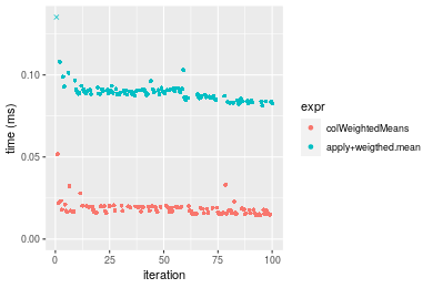
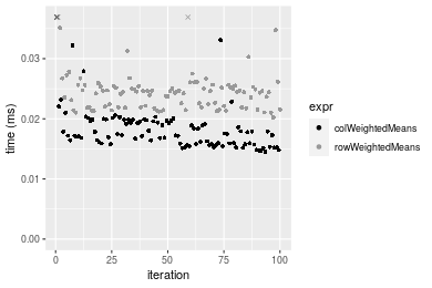
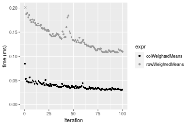
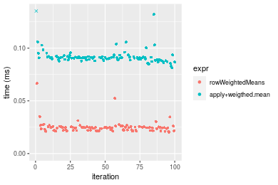Table: Benchmarking of colWeightedMeans() and rowWeightedMeans() on 10x10 data (original and transposed). The top panel shows times in milliseconds and the bottom panel shows relative times.

	expr	min	lq	mean	median	uq	max
1	colWeightedMeans	14.514	15.8945	18.37558	17.3735	19.6270	51.723
2	rowWeightedMeans	20.235	21.9355	24.88602	24.4995	25.3815	66.676

	expr	min	lq	mean	median	uq	max
1	colWeightedMeans	1.000000	1.000000	1.000000	1.000000	1.000000	1.000000
2	rowWeightedMeans	1.394171	1.380069	1.354299	1.410165	1.293193	1.289098

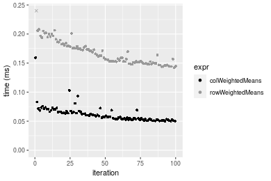
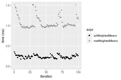
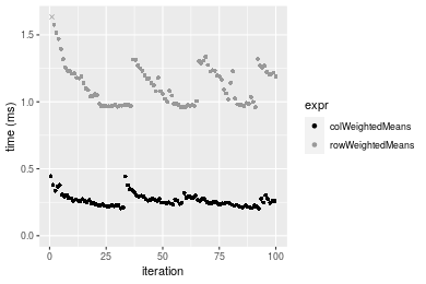
Figure: Benchmarking of colWeightedMeans() and rowWeightedMeans() on 10x10 data (original and transposed). Outliers are displayed as crosses. Times are in milliseconds.

100x100 matrix

> X <- data[["100x100"]]
> w <- runif(nrow(X))
> gc()
           used  (Mb) gc trigger  (Mb) max used  (Mb)
Ncells  5329664 284.7    7916910 422.9  7916910 422.9
Vcells 10469040  79.9   33191153 253.3 53339345 407.0
> colStats <- microbenchmark(colWeightedMeans = colWeightedMeans(X, w = w, na.rm = FALSE), `apply+weigthed.mean` = apply(X, 
+     MARGIN = 2L, FUN = weighted.mean, w = w, na.rm = FALSE), unit = "ms")
> X <- t(X)
> gc()
           used  (Mb) gc trigger  (Mb) max used  (Mb)
Ncells  5329658 284.7    7916910 422.9  7916910 422.9
Vcells 10479083  80.0   33191153 253.3 53339345 407.0
> rowStats <- microbenchmark(rowWeightedMeans = rowWeightedMeans(X, w = w, na.rm = FALSE), `apply+weigthed.mean` = apply(X, 
+     MARGIN = 1L, FUN = weighted.mean, w = w, na.rm = FALSE), unit = "ms")

Table: Benchmarking of colWeightedMeans() and apply+weigthed.mean() on 100x100 data. The top panel shows times in milliseconds and the bottom panel shows relative times.

	expr	min	lq	mean	median	uq	max
1	colWeightedMeans	0.030195	0.032921	0.0382298	0.03661	0.0418240	0.084657
2	apply+weigthed.mean	0.534847	0.554290	0.6471003	0.63325	0.7064345	1.068205

	expr	min	lq	mean	median	uq	max
1	colWeightedMeans	1.0000	1.00000	1.00000	1.00000	1.00000	1.00000
2	apply+weigthed.mean	17.7131	16.83697	16.92659	17.29719	16.89065	12.61804

Table: Benchmarking of rowWeightedMeans() and apply+weigthed.mean() on 100x100 data (transposed). The top panel shows times in milliseconds and the bottom panel shows relative times.

	expr	min	lq	mean	median	uq	max
1	rowWeightedMeans	0.108045	0.114521	0.1378237	0.1341905	0.1548515	0.224745
2	apply+weigthed.mean	0.535381	0.558136	0.6648594	0.6451205	0.7158065	1.127485

	expr	min	lq	mean	median	uq	max
1	rowWeightedMeans	1.000000	1.000000	1.000000	1.000000	1.000000	1.00000
2	apply+weigthed.mean	4.955167	4.873656	4.823984	4.807498	4.622535	5.01673

Figure: Benchmarking of colWeightedMeans() and apply+weigthed.mean() on 100x100 data as well as rowWeightedMeans() and apply+weigthed.mean() on the same data transposed. Outliers are displayed as crosses. Times are in milliseconds.

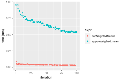
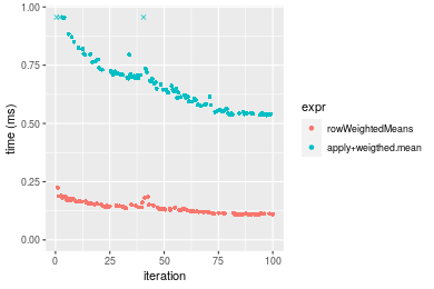Table: Benchmarking of colWeightedMeans() and rowWeightedMeans() on 100x100 data (original and transposed). The top panel shows times in milliseconds and the bottom panel shows relative times.

	expr	min	lq	mean	median	uq	max
1	colWeightedMeans	30.195	32.921	38.2298	36.6100	41.8240	84.657
2	rowWeightedMeans	108.045	114.521	137.8237	134.1905	154.8515	224.745

	expr	min	lq	mean	median	uq	max
1	colWeightedMeans	1.000000	1.000000	1.000000	1.000000	1.000000	1.000000
2	rowWeightedMeans	3.578241	3.478661	3.605138	3.665406	3.702456	2.654772

Figure: Benchmarking of colWeightedMeans() and rowWeightedMeans() on 100x100 data (original and transposed). Outliers are displayed as crosses. Times are in milliseconds.

1000x10 matrix

> X <- data[["1000x10"]]
> w <- runif(nrow(X))
> gc()
           used  (Mb) gc trigger  (Mb) max used  (Mb)
Ncells  5330389 284.7    7916910 422.9  7916910 422.9
Vcells 10473445  80.0   33191153 253.3 53339345 407.0
> colStats <- microbenchmark(colWeightedMeans = colWeightedMeans(X, w = w, na.rm = FALSE), `apply+weigthed.mean` = apply(X, 
+     MARGIN = 2L, FUN = weighted.mean, w = w, na.rm = FALSE), unit = "ms")
> X <- t(X)
> gc()
           used  (Mb) gc trigger  (Mb) max used  (Mb)
Ncells  5330377 284.7    7916910 422.9  7916910 422.9
Vcells 10483478  80.0   33191153 253.3 53339345 407.0
> rowStats <- microbenchmark(rowWeightedMeans = rowWeightedMeans(X, w = w, na.rm = FALSE), `apply+weigthed.mean` = apply(X, 
+     MARGIN = 1L, FUN = weighted.mean, w = w, na.rm = FALSE), unit = "ms")

Table: Benchmarking of colWeightedMeans() and apply+weigthed.mean() on 1000x10 data. The top panel shows times in milliseconds and the bottom panel shows relative times.

	expr	min	lq	mean	median	uq	max
1	colWeightedMeans	0.050207	0.052973	0.0616090	0.058177	0.0663215	0.159488
2	apply+weigthed.mean	0.207594	0.215316	0.2434847	0.231619	0.2656575	0.379112

	expr	min	lq	mean	median	uq	max
1	colWeightedMeans	1.000000	1.000000	1.000000	1.000000	1.000000	1.000000
2	apply+weigthed.mean	4.134762	4.064637	3.952096	3.981281	4.005602	2.377057

Table: Benchmarking of rowWeightedMeans() and apply+weigthed.mean() on 1000x10 data (transposed). The top panel shows times in milliseconds and the bottom panel shows relative times.

	expr	min	lq	mean	median	uq	max
1	rowWeightedMeans	0.142004	0.1511195	0.1673899	0.160325	0.179218	0.262431
2	apply+weigthed.mean	0.202047	0.2183060	0.2437231	0.236016	0.261967	0.353293

	expr	min	lq	mean	median	uq	max
1	rowWeightedMeans	1.000000	1.000000	1.00000	1.00000	1.000000	1.000000
2	apply+weigthed.mean	1.422826	1.444592	1.45602	1.47211	1.461723	1.346232

Figure: Benchmarking of colWeightedMeans() and apply+weigthed.mean() on 1000x10 data as well as rowWeightedMeans() and apply+weigthed.mean() on the same data transposed. Outliers are displayed as crosses. Times are in milliseconds.

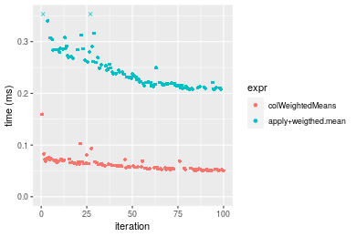
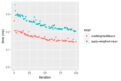Table: Benchmarking of colWeightedMeans() and rowWeightedMeans() on 1000x10 data (original and transposed). The top panel shows times in milliseconds and the bottom panel shows relative times.

	expr	min	lq	mean	median	uq	max
1	colWeightedMeans	50.207	52.9730	61.60899	58.177	66.3215	159.488
2	rowWeightedMeans	142.004	151.1195	167.38994	160.325	179.2180	262.431

	expr	min	lq	mean	median	uq	max
1	colWeightedMeans	1.000000	1.000000	1.000000	1.000000	1.000000	1.000000
2	rowWeightedMeans	2.828371	2.852765	2.716973	2.755814	2.702261	1.645459

Figure: Benchmarking of colWeightedMeans() and rowWeightedMeans() on 1000x10 data (original and transposed). Outliers are displayed as crosses. Times are in milliseconds.

10x1000 matrix

> X <- data[["10x1000"]]
> w <- runif(nrow(X))
> gc()
           used  (Mb) gc trigger  (Mb) max used  (Mb)
Ncells  5330581 284.7    7916910 422.9  7916910 422.9
Vcells 10473235  80.0   33191153 253.3 53339345 407.0
> colStats <- microbenchmark(colWeightedMeans = colWeightedMeans(X, w = w, na.rm = FALSE), `apply+weigthed.mean` = apply(X, 
+     MARGIN = 2L, FUN = weighted.mean, w = w, na.rm = FALSE), unit = "ms")
> X <- t(X)
> gc()
           used  (Mb) gc trigger  (Mb) max used  (Mb)
Ncells  5330575 284.7    7916910 422.9  7916910 422.9
Vcells 10483278  80.0   33191153 253.3 53339345 407.0
> rowStats <- microbenchmark(rowWeightedMeans = rowWeightedMeans(X, w = w, na.rm = FALSE), `apply+weigthed.mean` = apply(X, 
+     MARGIN = 1L, FUN = weighted.mean, w = w, na.rm = FALSE), unit = "ms")

Table: Benchmarking of colWeightedMeans() and apply+weigthed.mean() on 10x1000 data. The top panel shows times in milliseconds and the bottom panel shows relative times.

	expr	min	lq	mean	median	uq	max
1	colWeightedMeans	0.027890	0.031472	0.0402594	0.0373785	0.043889	0.100983
2	apply+weigthed.mean	4.093371	4.224227	4.6551195	4.3682620	4.654880	12.683915

	expr	min	lq	mean	median	uq	max
1	colWeightedMeans	1.0000	1.0000	1.0000	1.0000	1.0000	1.0000
2	apply+weigthed.mean	146.7684	134.2218	115.6281	116.8656	106.0603	125.6045

Table: Benchmarking of rowWeightedMeans() and apply+weigthed.mean() on 10x1000 data (transposed). The top panel shows times in milliseconds and the bottom panel shows relative times.

	expr	min	lq	mean	median	uq	max
1	rowWeightedMeans	0.106895	0.1135865	0.1268637	0.121555	0.1352205	0.223218
2	apply+weigthed.mean	4.066901	4.2600495	4.6186294	4.353472	4.5128765	11.151535

	expr	min	lq	mean	median	uq	max
1	rowWeightedMeans	1.00000	1.00000	1.00000	1.00000	1.0000	1.00000
2	apply+weigthed.mean	38.04576	37.50489	36.40624	35.81484	33.3742	49.95805

Figure: Benchmarking of colWeightedMeans() and apply+weigthed.mean() on 10x1000 data as well as rowWeightedMeans() and apply+weigthed.mean() on the same data transposed. Outliers are displayed as crosses. Times are in milliseconds.

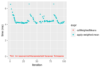
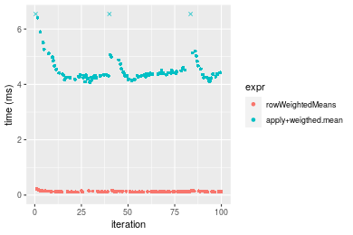Table: Benchmarking of colWeightedMeans() and rowWeightedMeans() on 10x1000 data (original and transposed). The top panel shows times in milliseconds and the bottom panel shows relative times.

	expr	min	lq	mean	median	uq	max
1	colWeightedMeans	27.890	31.4720	40.25943	37.3785	43.8890	100.983
2	rowWeightedMeans	106.895	113.5865	126.86366	121.5550	135.2205	223.218

	expr	min	lq	mean	median	uq	max
1	colWeightedMeans	1.000000	1.000000	1.000000	1.000000	1.000000	1.000000
2	rowWeightedMeans	3.832736	3.609129	3.151154	3.252003	3.080966	2.210451

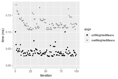
Figure: Benchmarking of colWeightedMeans() and rowWeightedMeans() on 10x1000 data (original and transposed). Outliers are displayed as crosses. Times are in milliseconds.

100x1000 matrix

> X <- data[["100x1000"]]
> w <- runif(nrow(X))
> gc()
           used  (Mb) gc trigger  (Mb) max used  (Mb)
Ncells  5330777 284.7    7916910 422.9  7916910 422.9
Vcells 10473841  80.0   33191153 253.3 53339345 407.0
> colStats <- microbenchmark(colWeightedMeans = colWeightedMeans(X, w = w, na.rm = FALSE), `apply+weigthed.mean` = apply(X, 
+     MARGIN = 2L, FUN = weighted.mean, w = w, na.rm = FALSE), unit = "ms")
> X <- t(X)
> gc()
           used  (Mb) gc trigger  (Mb) max used  (Mb)
Ncells  5330765 284.7    7916910 422.9  7916910 422.9
Vcells 10573874  80.7   33191153 253.3 53339345 407.0
> rowStats <- microbenchmark(rowWeightedMeans = rowWeightedMeans(X, w = w, na.rm = FALSE), `apply+weigthed.mean` = apply(X, 
+     MARGIN = 1L, FUN = weighted.mean, w = w, na.rm = FALSE), unit = "ms")

Table: Benchmarking of colWeightedMeans() and apply+weigthed.mean() on 100x1000 data. The top panel shows times in milliseconds and the bottom panel shows relative times.

	expr	min	lq	mean	median	uq	max
1	colWeightedMeans	0.176290	0.2078795	0.4456043	0.234187	0.270846	20.88489
2	apply+weigthed.mean	5.194491	5.3765175	6.1930076	5.488162	5.870243	27.26077

	expr	min	lq	mean	median	uq	max
1	colWeightedMeans	1.0000	1.00000	1.000	1.00000	1.00000	1.000000
2	apply+weigthed.mean	29.4656	25.86363	13.898	23.43496	21.67373	1.305286

Table: Benchmarking of rowWeightedMeans() and apply+weigthed.mean() on 100x1000 data (transposed). The top panel shows times in milliseconds and the bottom panel shows relative times.

	expr	min	lq	mean	median	uq	max
1	rowWeightedMeans	0.939194	0.9811385	1.280713	1.007786	1.164391	22.33007
2	apply+weigthed.mean	5.244182	5.3788310	6.250966	5.525034	5.953479	28.91215

	expr	min	lq	mean	median	uq	max
1	rowWeightedMeans	1.000000	1.000000	1.000000	1.000000	1.000000	1.000000
2	apply+weigthed.mean	5.583705	5.482234	4.880847	5.482348	5.112957	1.294763

Figure: Benchmarking of colWeightedMeans() and apply+weigthed.mean() on 100x1000 data as well as rowWeightedMeans() and apply+weigthed.mean() on the same data transposed. Outliers are displayed as crosses. Times are in milliseconds.

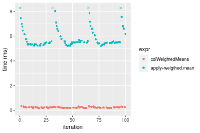
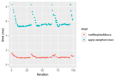Table: Benchmarking of colWeightedMeans() and rowWeightedMeans() on 100x1000 data (original and transposed). The top panel shows times in milliseconds and the bottom panel shows relative times.

	expr	min	lq	mean	median	uq	max
1	colWeightedMeans	176.290	207.8795	445.6043	234.187	270.846	20884.89
2	rowWeightedMeans	939.194	981.1385	1280.7132	1007.786	1164.390	22330.07

	expr	min	lq	mean	median	uq	max
1	colWeightedMeans	1.000000	1.000000	1.000000	1.000000	1.000000	1.000000
2	rowWeightedMeans	5.327551	4.719746	2.874104	4.303339	4.299087	1.069197

Figure: Benchmarking of colWeightedMeans() and rowWeightedMeans() on 100x1000 data (original and transposed). Outliers are displayed as crosses. Times are in milliseconds.

1000x100 matrix

> X <- data[["1000x100"]]
> w <- runif(nrow(X))
> gc()
           used  (Mb) gc trigger  (Mb) max used  (Mb)
Ncells  5330958 284.8    7916910 422.9  7916910 422.9
Vcells 10475373  80.0   33191153 253.3 53339345 407.0
> colStats <- microbenchmark(colWeightedMeans = colWeightedMeans(X, w = w, na.rm = FALSE), `apply+weigthed.mean` = apply(X, 
+     MARGIN = 2L, FUN = weighted.mean, w = w, na.rm = FALSE), unit = "ms")
> X <- t(X)
> gc()
           used  (Mb) gc trigger  (Mb) max used  (Mb)
Ncells  5330952 284.8    7916910 422.9  7916910 422.9
Vcells 10575416  80.7   33191153 253.3 53339345 407.0
> rowStats <- microbenchmark(rowWeightedMeans = rowWeightedMeans(X, w = w, na.rm = FALSE), `apply+weigthed.mean` = apply(X, 
+     MARGIN = 1L, FUN = weighted.mean, w = w, na.rm = FALSE), unit = "ms")

Table: Benchmarking of colWeightedMeans() and apply+weigthed.mean() on 1000x100 data. The top panel shows times in milliseconds and the bottom panel shows relative times.

	expr	min	lq	mean	median	uq	max
1	colWeightedMeans	0.201873	0.2324025	0.2648283	0.2548875	0.281130	0.443784
2	apply+weigthed.mean	1.514922	1.6610620	5.8543197	1.8988915	2.089488	376.589480

	expr	min	lq	mean	median	uq	max
1	colWeightedMeans	1.000000	1.00000	1.00000	1.00000	1.000000	1.0000
2	apply+weigthed.mean	7.504332	7.14735	22.10609	7.44992	7.432464	848.5873

Table: Benchmarking of rowWeightedMeans() and apply+weigthed.mean() on 1000x100 data (transposed). The top panel shows times in milliseconds and the bottom panel shows relative times.

	expr	min	lq	mean	median	uq	max
1	rowWeightedMeans	0.959981	0.979435	1.125434	1.090402	1.228889	1.656196
2	apply+weigthed.mean	1.523706	1.564525	2.017792	1.617954	1.943826	11.460256

	expr	min	lq	mean	median	uq	max
1	rowWeightedMeans	1.000000	1.000000	1.000000	1.000000	1.000000	1.000000
2	apply+weigthed.mean	1.587225	1.597374	1.792902	1.483814	1.581775	6.919626

Figure: Benchmarking of colWeightedMeans() and apply+weigthed.mean() on 1000x100 data as well as rowWeightedMeans() and apply+weigthed.mean() on the same data transposed. Outliers are displayed as crosses. Times are in milliseconds.

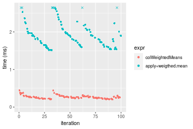
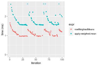Table: Benchmarking of colWeightedMeans() and rowWeightedMeans() on 1000x100 data (original and transposed). The top panel shows times in milliseconds and the bottom panel shows relative times.

	expr	min	lq	mean	median	uq	max
1	colWeightedMeans	201.873	232.4025	264.8283	254.8875	281.130	443.784
2	rowWeightedMeans	959.981	979.4350	1125.4340	1090.4015	1228.889	1656.196

	expr	min	lq	mean	median	uq	max
1	colWeightedMeans	1.000000	1.000000	1.000000	1.000000	1.000000	1.000000
2	rowWeightedMeans	4.755371	4.214391	4.249674	4.277972	4.371248	3.731987

Figure: Benchmarking of colWeightedMeans() and rowWeightedMeans() on 1000x100 data (original and transposed). Outliers are displayed as crosses. Times are in milliseconds.

Appendix

Session information

R version 4.1.1 Patched (2021-08-10 r80727)
Platform: x86_64-pc-linux-gnu (64-bit)
Running under: Ubuntu 18.04.5 LTS

Matrix products: default
BLAS:   /home/hb/software/R-devel/R-4-1-branch/lib/R/lib/libRblas.so
LAPACK: /home/hb/software/R-devel/R-4-1-branch/lib/R/lib/libRlapack.so

locale:
 [1] LC_CTYPE=en_US.UTF-8       LC_NUMERIC=C              
 [3] LC_TIME=en_US.UTF-8        LC_COLLATE=en_US.UTF-8    
 [5] LC_MONETARY=en_US.UTF-8    LC_MESSAGES=en_US.UTF-8   
 [7] LC_PAPER=en_US.UTF-8       LC_NAME=C                 
 [9] LC_ADDRESS=C               LC_TELEPHONE=C            
[11] LC_MEASUREMENT=en_US.UTF-8 LC_IDENTIFICATION=C       

attached base packages:
[1] stats     graphics  grDevices utils     datasets  methods   base     

other attached packages:
[1] microbenchmark_1.4-7   matrixStats_0.60.0     ggplot2_3.3.5         
[4] knitr_1.33             R.devices_2.17.0       R.utils_2.10.1        
[7] R.oo_1.24.0            R.methodsS3_1.8.1-9001 history_0.0.1-9000    

loaded via a namespace (and not attached):
 [1] Biobase_2.52.0          httr_1.4.2              splines_4.1.1          
 [4] bit64_4.0.5             network_1.17.1          assertthat_0.2.1       
 [7] highr_0.9               stats4_4.1.1            blob_1.2.2             
[10] GenomeInfoDbData_1.2.6  robustbase_0.93-8       pillar_1.6.2           
[13] RSQLite_2.2.8           lattice_0.20-44         glue_1.4.2             
[16] digest_0.6.27           XVector_0.32.0          colorspace_2.0-2       
[19] Matrix_1.3-4            XML_3.99-0.7            pkgconfig_2.0.3        
[22] zlibbioc_1.38.0         genefilter_1.74.0       purrr_0.3.4            
[25] ergm_4.1.2              xtable_1.8-4            scales_1.1.1           
[28] tibble_3.1.4            annotate_1.70.0         KEGGREST_1.32.0        
[31] farver_2.1.0            generics_0.1.0          IRanges_2.26.0         
[34] ellipsis_0.3.2          cachem_1.0.6            withr_2.4.2            
[37] BiocGenerics_0.38.0     mime_0.11               survival_3.2-13        
[40] magrittr_2.0.1          crayon_1.4.1            statnet.common_4.5.0   
[43] memoise_2.0.0           laeken_0.5.1            fansi_0.5.0            
[46] R.cache_0.15.0          MASS_7.3-54             R.rsp_0.44.0           
[49] progressr_0.8.0         tools_4.1.1             lifecycle_1.0.0        
[52] S4Vectors_0.30.0        trust_0.1-8             munsell_0.5.0          
[55] tabby_0.0.1-9001        AnnotationDbi_1.54.1    Biostrings_2.60.2      
[58] compiler_4.1.1          GenomeInfoDb_1.28.1     rlang_0.4.11           
[61] grid_4.1.1              RCurl_1.98-1.4          cwhmisc_6.6            
[64] rstudioapi_0.13         rappdirs_0.3.3          startup_0.15.0         
[67] labeling_0.4.2          bitops_1.0-7            base64enc_0.1-3        
[70] boot_1.3-28             gtable_0.3.0            DBI_1.1.1              
[73] markdown_1.1            R6_2.5.1                lpSolveAPI_5.5.2.0-17.7
[76] rle_0.9.2               dplyr_1.0.7             fastmap_1.1.0          
[79] bit_4.0.4               utf8_1.2.2              parallel_4.1.1         
[82] Rcpp_1.0.7              vctrs_0.3.8             png_0.1-7              
[85] DEoptimR_1.0-9          tidyselect_1.1.1        xfun_0.25              
[88] coda_0.19-4            

Total processing time was 15.44 secs.

Reproducibility

To reproduce this report, do:

html <- matrixStats:::benchmark('colWeightedMeans')

---

Copyright Henrik Bengtsson. Last updated on 2021-08-25 22:32:10 (+0200 UTC). Powered by RSP.