matrixStats.benchmarks
colRanges() and rowRanges() benchmarks
This report benchmark the performance of colRanges() and rowRanges() against alternative methods.
Alternative methods
- apply() + range()
Data type “integer”
Data
> rmatrix <- function(nrow, ncol, mode = c("logical", "double", "integer", "index"), range = c(-100,
+     +100), na_prob = 0) {
+     mode <- match.arg(mode)
+     n <- nrow * ncol
+     if (mode == "logical") {
+         x <- sample(c(FALSE, TRUE), size = n, replace = TRUE)
+     }     else if (mode == "index") {
+         x <- seq_len(n)
+         mode <- "integer"
+     }     else {
+         x <- runif(n, min = range[1], max = range[2])
+     }
+     storage.mode(x) <- mode
+     if (na_prob > 0)
+         x[sample(n, size = na_prob * n)] <- NA
+     dim(x) <- c(nrow, ncol)
+     x
+ }
> rmatrices <- function(scale = 10, seed = 1, ...) {
+     set.seed(seed)
+     data <- list()
+     data[[1]] <- rmatrix(nrow = scale * 1, ncol = scale * 1, ...)
+     data[[2]] <- rmatrix(nrow = scale * 10, ncol = scale * 10, ...)
+     data[[3]] <- rmatrix(nrow = scale * 100, ncol = scale * 1, ...)
+     data[[4]] <- t(data[[3]])
+     data[[5]] <- rmatrix(nrow = scale * 10, ncol = scale * 100, ...)
+     data[[6]] <- t(data[[5]])
+     names(data) <- sapply(data, FUN = function(x) paste(dim(x), collapse = "x"))
+     data
+ }
> data <- rmatrices(mode = mode)
Results
10x10 integer matrix
> X <- data[["10x10"]]
> gc()
           used  (Mb) gc trigger  (Mb) max used  (Mb)
Ncells  5290711 282.6    7916910 422.9  7916910 422.9
Vcells 10476589  80.0   33191153 253.3 53339345 407.0
> colStats <- microbenchmark(colRanges = colRanges(X, na.rm = FALSE), `apply+range` = apply(X, MARGIN = 2L,
+     FUN = range, na.rm = FALSE), unit = "ms")
> X <- t(X)
> gc()
           used  (Mb) gc trigger  (Mb) max used  (Mb)
Ncells  5290306 282.6    7916910 422.9  7916910 422.9
Vcells 10475612  80.0   33191153 253.3 53339345 407.0
> rowStats <- microbenchmark(rowRanges = rowRanges(X, na.rm = FALSE), `apply+range` = apply(X, MARGIN = 1L,
+     FUN = range, na.rm = FALSE), unit = "ms")
Table: Benchmarking of colRanges() and apply+range() on integer+10x10 data. The top panel shows times in milliseconds and the bottom panel shows relative times.
| expr | min | lq | mean | median | uq | max | |
|---|---|---|---|---|---|---|---|
| 1 | colRanges | 0.002473 | 0.002782 | 0.0036021 | 0.0030815 | 0.0041665 | 0.016364 |
| 2 | apply+range | 0.061796 | 0.063297 | 0.0673617 | 0.0647410 | 0.0672345 | 0.165235 |
| expr | min | lq | mean | median | uq | max | |
|---|---|---|---|---|---|---|---|
| 1 | colRanges | 1.00000 | 1.00000 | 1.00000 | 1.00000 | 1.00000 | 1.00000 |
| 2 | apply+range | 24.98827 | 22.75234 | 18.70048 | 21.00957 | 16.13693 | 10.09747 |
Table: Benchmarking of rowRanges() and apply+range() on integer+10x10 data (transposed). The top panel shows times in milliseconds and the bottom panel shows relative times.
| expr | min | lq | mean | median | uq | max | |
|---|---|---|---|---|---|---|---|
| 1 | rowRanges | 0.002468 | 0.0029030 | 0.0038761 | 0.0040395 | 0.004299 | 0.016288 |
| 2 | apply+range | 0.061815 | 0.0630775 | 0.0670372 | 0.0641105 | 0.067389 | 0.163298 |
| expr | min | lq | mean | median | uq | max | |
|---|---|---|---|---|---|---|---|
| 1 | rowRanges | 1.0000 | 1.00000 | 1.00000 | 1.0000 | 1.00000 | 1.00000 |
| 2 | apply+range | 25.0466 | 21.72838 | 17.29502 | 15.8709 | 15.67551 | 10.02566 |
Figure: Benchmarking of colRanges() and apply+range() on integer+10x10 data as well as rowRanges() and apply+range() on the same data transposed. Outliers are displayed as crosses. Times are in milliseconds.
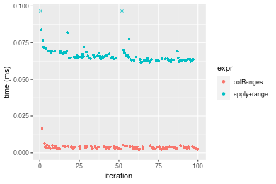
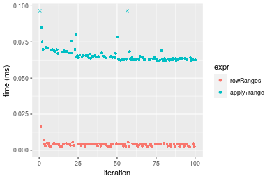 Table: Benchmarking of colRanges() and rowRanges() on integer+10x10 data (original and transposed). The top panel shows times in milliseconds and the bottom panel shows relative times.
| expr | min | lq | mean | median | uq | max | |
|---|---|---|---|---|---|---|---|
| 1 | colRanges | 2.473 | 2.782 | 3.60214 | 3.0815 | 4.1665 | 16.364 |
| 2 | rowRanges | 2.468 | 2.903 | 3.87610 | 4.0395 | 4.2990 | 16.288 |
| expr | min | lq | mean | median | uq | max | |
|---|---|---|---|---|---|---|---|
| 1 | colRanges | 1.0000000 | 1.000000 | 1.000000 | 1.000000 | 1.000000 | 1.0000000 |
| 2 | rowRanges | 0.9979782 | 1.043494 | 1.076055 | 1.310888 | 1.031801 | 0.9953557 |
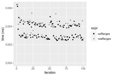
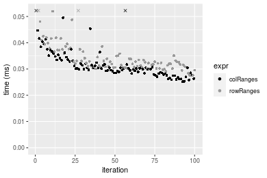
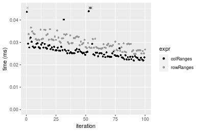
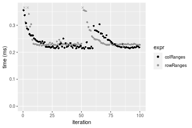
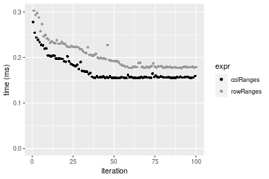
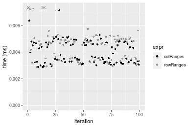
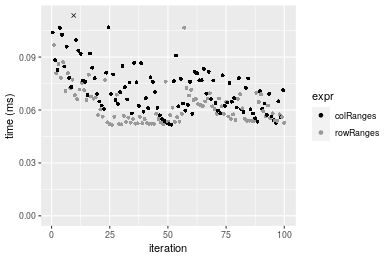
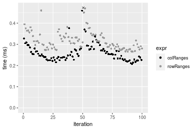
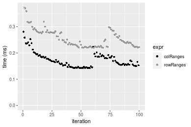
Figure: Benchmarking of colRanges() and rowRanges() on integer+10x10 data (original and transposed). Outliers are displayed as crosses. Times are in milliseconds.
100x100 integer matrix
> X <- data[["100x100"]]
> gc()
           used  (Mb) gc trigger  (Mb) max used  (Mb)
Ncells  5288866 282.5    7916910 422.9  7916910 422.9
Vcells 10092114  77.0   33191153 253.3 53339345 407.0
> colStats <- microbenchmark(colRanges = colRanges(X, na.rm = FALSE), `apply+range` = apply(X, MARGIN = 2L,
+     FUN = range, na.rm = FALSE), unit = "ms")
> X <- t(X)
> gc()
           used  (Mb) gc trigger  (Mb) max used  (Mb)
Ncells  5288860 282.5    7916910 422.9  7916910 422.9
Vcells 10097157  77.1   33191153 253.3 53339345 407.0
> rowStats <- microbenchmark(rowRanges = rowRanges(X, na.rm = FALSE), `apply+range` = apply(X, MARGIN = 1L,
+     FUN = range, na.rm = FALSE), unit = "ms")
Table: Benchmarking of colRanges() and apply+range() on integer+100x100 data. The top panel shows times in milliseconds and the bottom panel shows relative times.
| expr | min | lq | mean | median | uq | max | |
|---|---|---|---|---|---|---|---|
| 1 | colRanges | 0.025231 | 0.0285145 | 0.0320065 | 0.0301910 | 0.033218 | 0.079283 |
| 2 | apply+range | 0.374070 | 0.4097785 | 0.4503690 | 0.4266275 | 0.488610 | 0.667680 |
| expr | min | lq | mean | median | uq | max | |
|---|---|---|---|---|---|---|---|
| 1 | colRanges | 1.00000 | 1.00000 | 1.00000 | 1.00000 | 1.00000 | 1.000000 |
| 2 | apply+range | 14.82581 | 14.37088 | 14.07116 | 14.13095 | 14.70919 | 8.421477 |
Table: Benchmarking of rowRanges() and apply+range() on integer+100x100 data (transposed). The top panel shows times in milliseconds and the bottom panel shows relative times.
| expr | min | lq | mean | median | uq | max | |
|---|---|---|---|---|---|---|---|
| 1 | rowRanges | 0.027509 | 0.0307135 | 0.0349542 | 0.0324365 | 0.0366515 | 0.087596 |
| 2 | apply+range | 0.387839 | 0.4097395 | 0.4576021 | 0.4304910 | 0.4923930 | 0.732246 |
| expr | min | lq | mean | median | uq | max | |
|---|---|---|---|---|---|---|---|
| 1 | rowRanges | 1.00000 | 1.0000 | 1.00000 | 1.00000 | 1.00000 | 1.000000 |
| 2 | apply+range | 14.09862 | 13.3407 | 13.09146 | 13.27181 | 13.43446 | 8.359354 |
Figure: Benchmarking of colRanges() and apply+range() on integer+100x100 data as well as rowRanges() and apply+range() on the same data transposed. Outliers are displayed as crosses. Times are in milliseconds.
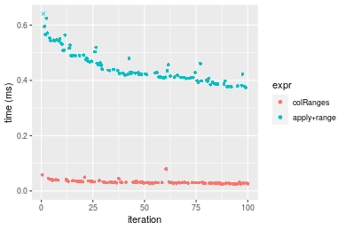
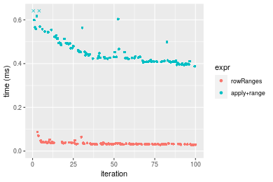 Table: Benchmarking of colRanges() and rowRanges() on integer+100x100 data (original and transposed). The top panel shows times in milliseconds and the bottom panel shows relative times.
| expr | min | lq | mean | median | uq | max | |
|---|---|---|---|---|---|---|---|
| 1 | colRanges | 25.231 | 28.5145 | 32.00652 | 30.1910 | 33.2180 | 79.283 |
| 2 | rowRanges | 27.509 | 30.7135 | 34.95425 | 32.4365 | 36.6515 | 87.596 |
| expr | min | lq | mean | median | uq | max | |
|---|---|---|---|---|---|---|---|
| 1 | colRanges | 1.000000 | 1.000000 | 1.000000 | 1.000000 | 1.000000 | 1.000000 |
| 2 | rowRanges | 1.090286 | 1.077119 | 1.092098 | 1.074377 | 1.103363 | 1.104852 |
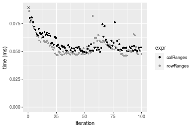
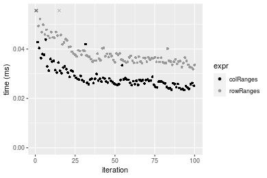
Figure: Benchmarking of colRanges() and rowRanges() on integer+100x100 data (original and transposed). Outliers are displayed as crosses. Times are in milliseconds.
1000x10 integer matrix
> X <- data[["1000x10"]]
> gc()
           used  (Mb) gc trigger  (Mb) max used  (Mb)
Ncells  5289602 282.5    7916910 422.9  7916910 422.9
Vcells 10095627  77.1   33191153 253.3 53339345 407.0
> colStats <- microbenchmark(colRanges = colRanges(X, na.rm = FALSE), `apply+range` = apply(X, MARGIN = 2L,
+     FUN = range, na.rm = FALSE), unit = "ms")
> X <- t(X)
> gc()
           used  (Mb) gc trigger  (Mb) max used  (Mb)
Ncells  5289590 282.5    7916910 422.9  7916910 422.9
Vcells 10100660  77.1   33191153 253.3 53339345 407.0
> rowStats <- microbenchmark(rowRanges = rowRanges(X, na.rm = FALSE), `apply+range` = apply(X, MARGIN = 1L,
+     FUN = range, na.rm = FALSE), unit = "ms")
Table: Benchmarking of colRanges() and apply+range() on integer+1000x10 data. The top panel shows times in milliseconds and the bottom panel shows relative times.
| expr | min | lq | mean | median | uq | max | |
|---|---|---|---|---|---|---|---|
| 1 | colRanges | 0.021882 | 0.023777 | 0.0266113 | 0.0255570 | 0.027650 | 0.050962 |
| 2 | apply+range | 0.158220 | 0.171353 | 0.1913571 | 0.1858885 | 0.200442 | 0.364808 |
| expr | min | lq | mean | median | uq | max | |
|---|---|---|---|---|---|---|---|
| 1 | colRanges | 1.000000 | 1.00000 | 1.000000 | 1.000000 | 1.000000 | 1.000000 |
| 2 | apply+range | 7.230601 | 7.20667 | 7.190815 | 7.273487 | 7.249259 | 7.158432 |
Table: Benchmarking of rowRanges() and apply+range() on integer+1000x10 data (transposed). The top panel shows times in milliseconds and the bottom panel shows relative times.
| expr | min | lq | mean | median | uq | max | |
|---|---|---|---|---|---|---|---|
| 1 | rowRanges | 0.024865 | 0.0274885 | 0.0300131 | 0.029600 | 0.0318100 | 0.048732 |
| 2 | apply+range | 0.158219 | 0.1735090 | 0.1857822 | 0.182612 | 0.1987155 | 0.287092 |
| expr | min | lq | mean | median | uq | max | |
|---|---|---|---|---|---|---|---|
| 1 | rowRanges | 1.000000 | 1.000000 | 1.000000 | 1.000000 | 1.000000 | 1.000000 |
| 2 | apply+range | 6.363121 | 6.312058 | 6.190035 | 6.169324 | 6.246951 | 5.891242 |
Figure: Benchmarking of colRanges() and apply+range() on integer+1000x10 data as well as rowRanges() and apply+range() on the same data transposed. Outliers are displayed as crosses. Times are in milliseconds.
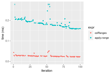
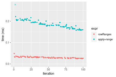 Table: Benchmarking of colRanges() and rowRanges() on integer+1000x10 data (original and transposed). The top panel shows times in milliseconds and the bottom panel shows relative times.
| expr | min | lq | mean | median | uq | max | |
|---|---|---|---|---|---|---|---|
| 1 | colRanges | 21.882 | 23.7770 | 26.61132 | 25.557 | 27.65 | 50.962 |
| 2 | rowRanges | 24.865 | 27.4885 | 30.01311 | 29.600 | 31.81 | 48.732 |
| expr | min | lq | mean | median | uq | max | |
|---|---|---|---|---|---|---|---|
| 1 | colRanges | 1.000000 | 1.000000 | 1.000000 | 1.000000 | 1.000000 | 1.0000000 |
| 2 | rowRanges | 1.136322 | 1.156096 | 1.127832 | 1.158195 | 1.150452 | 0.9562419 |
Figure: Benchmarking of colRanges() and rowRanges() on integer+1000x10 data (original and transposed). Outliers are displayed as crosses. Times are in milliseconds.
10x1000 integer matrix
> X <- data[["10x1000"]]
> gc()
           used  (Mb) gc trigger  (Mb) max used  (Mb)
Ncells  5289784 282.6    7916910 422.9  7916910 422.9
Vcells 10096288  77.1   33191153 253.3 53339345 407.0
> colStats <- microbenchmark(colRanges = colRanges(X, na.rm = FALSE), `apply+range` = apply(X, MARGIN = 2L,
+     FUN = range, na.rm = FALSE), unit = "ms")
> X <- t(X)
> gc()
           used  (Mb) gc trigger  (Mb) max used  (Mb)
Ncells  5289778 282.6    7916910 422.9  7916910 422.9
Vcells 10101331  77.1   33191153 253.3 53339345 407.0
> rowStats <- microbenchmark(rowRanges = rowRanges(X, na.rm = FALSE), `apply+range` = apply(X, MARGIN = 1L,
+     FUN = range, na.rm = FALSE), unit = "ms")
Table: Benchmarking of colRanges() and apply+range() on integer+10x1000 data. The top panel shows times in milliseconds and the bottom panel shows relative times.
| expr | min | lq | mean | median | uq | max | |
|---|---|---|---|---|---|---|---|
| 1 | colRanges | 0.048760 | 0.0515365 | 0.0574253 | 0.0539435 | 0.0624505 | 0.093977 |
| 2 | apply+range | 2.286009 | 2.3110690 | 2.5454226 | 2.3890505 | 2.5688840 | 8.147520 |
| expr | min | lq | mean | median | uq | max | |
|---|---|---|---|---|---|---|---|
| 1 | colRanges | 1.00000 | 1.00000 | 1.00000 | 1.00000 | 1.00000 | 1.00000 |
| 2 | apply+range | 46.88288 | 44.84334 | 44.32583 | 44.28801 | 41.13472 | 86.69696 |
Table: Benchmarking of rowRanges() and apply+range() on integer+10x1000 data (transposed). The top panel shows times in milliseconds and the bottom panel shows relative times.
| expr | min | lq | mean | median | uq | max | |
|---|---|---|---|---|---|---|---|
| 1 | rowRanges | 0.045986 | 0.048111 | 0.054664 | 0.051825 | 0.0588115 | 0.086165 |
| 2 | apply+range | 2.239152 | 2.324964 | 2.571745 | 2.401298 | 2.6230155 | 8.277417 |
| expr | min | lq | mean | median | uq | max | |
|---|---|---|---|---|---|---|---|
| 1 | rowRanges | 1.00000 | 1.000 | 1.00000 | 1.00000 | 1.00000 | 1.00000 |
| 2 | apply+range | 48.69204 | 48.325 | 47.04642 | 46.33475 | 44.60038 | 96.06472 |
Figure: Benchmarking of colRanges() and apply+range() on integer+10x1000 data as well as rowRanges() and apply+range() on the same data transposed. Outliers are displayed as crosses. Times are in milliseconds.
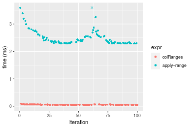
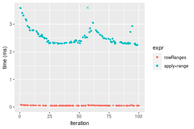 Table: Benchmarking of colRanges() and rowRanges() on integer+10x1000 data (original and transposed). The top panel shows times in milliseconds and the bottom panel shows relative times.
| expr | min | lq | mean | median | uq | max | |
|---|---|---|---|---|---|---|---|
| 2 | rowRanges | 45.986 | 48.1110 | 54.66398 | 51.8250 | 58.8115 | 86.165 |
| 1 | colRanges | 48.760 | 51.5365 | 57.42527 | 53.9435 | 62.4505 | 93.977 |
| expr | min | lq | mean | median | uq | max | |
|---|---|---|---|---|---|---|---|
| 2 | rowRanges | 1.000000 | 1.0000 | 1.000000 | 1.000000 | 1.000000 | 1.000000 |
| 1 | colRanges | 1.060323 | 1.0712 | 1.050514 | 1.040878 | 1.061876 | 1.090663 |
Figure: Benchmarking of colRanges() and rowRanges() on integer+10x1000 data (original and transposed). Outliers are displayed as crosses. Times are in milliseconds.
100x1000 integer matrix
> X <- data[["100x1000"]]
> gc()
           used  (Mb) gc trigger  (Mb) max used  (Mb)
Ncells  5289980 282.6    7916910 422.9  7916910 422.9
Vcells 10096785  77.1   33191153 253.3 53339345 407.0
> colStats <- microbenchmark(colRanges = colRanges(X, na.rm = FALSE), `apply+range` = apply(X, MARGIN = 2L,
+     FUN = range, na.rm = FALSE), unit = "ms")
> X <- t(X)
> gc()
           used  (Mb) gc trigger  (Mb) max used  (Mb)
Ncells  5289962 282.6    7916910 422.9  7916910 422.9
Vcells 10146808  77.5   33191153 253.3 53339345 407.0
> rowStats <- microbenchmark(rowRanges = rowRanges(X, na.rm = FALSE), `apply+range` = apply(X, MARGIN = 1L,
+     FUN = range, na.rm = FALSE), unit = "ms")
Table: Benchmarking of colRanges() and apply+range() on integer+100x1000 data. The top panel shows times in milliseconds and the bottom panel shows relative times.
| expr | min | lq | mean | median | uq | max | |
|---|---|---|---|---|---|---|---|
| 1 | colRanges | 0.213473 | 0.218363 | 0.2367702 | 0.223724 | 0.2457605 | 0.355539 |
| 2 | apply+range | 3.030555 | 3.097857 | 3.4724992 | 3.166438 | 3.3794380 | 18.319767 |
| expr | min | lq | mean | median | uq | max | |
|---|---|---|---|---|---|---|---|
| 1 | colRanges | 1.00000 | 1.00000 | 1.00000 | 1.00000 | 1.00000 | 1.00000 |
| 2 | apply+range | 14.19643 | 14.18673 | 14.66612 | 14.15332 | 13.75094 | 51.52674 |
Table: Benchmarking of rowRanges() and apply+range() on integer+100x1000 data (transposed). The top panel shows times in milliseconds and the bottom panel shows relative times.
| expr | min | lq | mean | median | uq | max | |
|---|---|---|---|---|---|---|---|
| 1 | rowRanges | 0.224587 | 0.2279005 | 0.2460298 | 0.2299505 | 0.2401315 | 0.387467 |
| 2 | apply+range | 3.043226 | 3.0889425 | 3.6265368 | 3.1390335 | 3.4800580 | 26.799406 |
| expr | min | lq | mean | median | uq | max | |
|---|---|---|---|---|---|---|---|
| 1 | rowRanges | 1.00000 | 1.00000 | 1.00000 | 1.00000 | 1.0000 | 1.00000 |
| 2 | apply+range | 13.55032 | 13.55391 | 14.74023 | 13.65091 | 14.4923 | 69.16565 |
Figure: Benchmarking of colRanges() and apply+range() on integer+100x1000 data as well as rowRanges() and apply+range() on the same data transposed. Outliers are displayed as crosses. Times are in milliseconds.
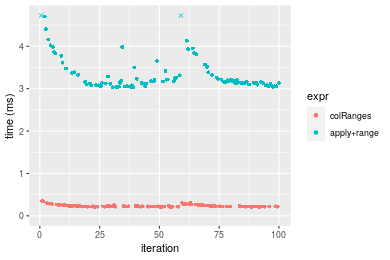
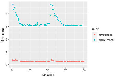 Table: Benchmarking of colRanges() and rowRanges() on integer+100x1000 data (original and transposed). The top panel shows times in milliseconds and the bottom panel shows relative times.
| expr | min | lq | mean | median | uq | max | |
|---|---|---|---|---|---|---|---|
| 1 | colRanges | 213.473 | 218.3630 | 236.7702 | 223.7240 | 245.7605 | 355.539 |
| 2 | rowRanges | 224.587 | 227.9005 | 246.0298 | 229.9505 | 240.1315 | 387.467 |
| expr | min | lq | mean | median | uq | max | |
|---|---|---|---|---|---|---|---|
| 1 | colRanges | 1.000000 | 1.000000 | 1.000000 | 1.000000 | 1.0000000 | 1.000000 |
| 2 | rowRanges | 1.052063 | 1.043677 | 1.039108 | 1.027831 | 0.9770956 | 1.089802 |
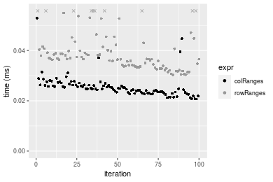
Figure: Benchmarking of colRanges() and rowRanges() on integer+100x1000 data (original and transposed). Outliers are displayed as crosses. Times are in milliseconds.
1000x100 integer matrix
> X <- data[["1000x100"]]
> gc()
           used  (Mb) gc trigger  (Mb) max used  (Mb)
Ncells  5290172 282.6    7916910 422.9  7916910 422.9
Vcells 10097343  77.1   33191153 253.3 53339345 407.0
> colStats <- microbenchmark(colRanges = colRanges(X, na.rm = FALSE), `apply+range` = apply(X, MARGIN = 2L,
+     FUN = range, na.rm = FALSE), unit = "ms")
> X <- t(X)
> gc()
           used  (Mb) gc trigger  (Mb) max used  (Mb)
Ncells  5290154 282.6    7916910 422.9  7916910 422.9
Vcells 10147366  77.5   33191153 253.3 53339345 407.0
> rowStats <- microbenchmark(rowRanges = rowRanges(X, na.rm = FALSE), `apply+range` = apply(X, MARGIN = 1L,
+     FUN = range, na.rm = FALSE), unit = "ms")
Table: Benchmarking of colRanges() and apply+range() on integer+1000x100 data. The top panel shows times in milliseconds and the bottom panel shows relative times.
| expr | min | lq | mean | median | uq | max | |
|---|---|---|---|---|---|---|---|
| 1 | colRanges | 0.154839 | 0.155973 | 0.1723323 | 0.157236 | 0.1852475 | 0.277939 |
| 2 | apply+range | 1.009848 | 1.019756 | 1.1499305 | 1.031660 | 1.2281775 | 1.818271 |
| expr | min | lq | mean | median | uq | max | |
|---|---|---|---|---|---|---|---|
| 1 | colRanges | 1.000000 | 1.000000 | 1.00000 | 1.00000 | 1.000000 | 1.000000 |
| 2 | apply+range | 6.521923 | 6.538032 | 6.67275 | 6.56122 | 6.629927 | 6.541979 |
Table: Benchmarking of rowRanges() and apply+range() on integer+1000x100 data (transposed). The top panel shows times in milliseconds and the bottom panel shows relative times.
| expr | min | lq | mean | median | uq | max | |
|---|---|---|---|---|---|---|---|
| 1 | rowRanges | 0.176820 | 0.1792245 | 0.2032811 | 0.192065 | 0.2231835 | 0.302751 |
| 2 | apply+range | 1.006984 | 1.0160345 | 1.1601044 | 1.032503 | 1.2505930 | 1.839541 |
| expr | min | lq | mean | median | uq | max | |
|---|---|---|---|---|---|---|---|
| 1 | rowRanges | 1.000000 | 1.00000 | 1.000000 | 1.0000 | 1.000000 | 1.000000 |
| 2 | apply+range | 5.694967 | 5.66906 | 5.706898 | 5.3758 | 5.603429 | 6.076086 |
Figure: Benchmarking of colRanges() and apply+range() on integer+1000x100 data as well as rowRanges() and apply+range() on the same data transposed. Outliers are displayed as crosses. Times are in milliseconds.
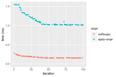
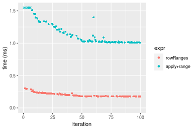 Table: Benchmarking of colRanges() and rowRanges() on integer+1000x100 data (original and transposed). The top panel shows times in milliseconds and the bottom panel shows relative times.
| expr | min | lq | mean | median | uq | max | |
|---|---|---|---|---|---|---|---|
| 1 | colRanges | 154.839 | 155.9730 | 172.3323 | 157.236 | 185.2475 | 277.939 |
| 2 | rowRanges | 176.820 | 179.2245 | 203.2811 | 192.065 | 223.1835 | 302.751 |
| expr | min | lq | mean | median | uq | max | |
|---|---|---|---|---|---|---|---|
| 1 | colRanges | 1.00000 | 1.000000 | 1.000000 | 1.000000 | 1.000000 | 1.000000 |
| 2 | rowRanges | 1.14196 | 1.149074 | 1.179588 | 1.221508 | 1.204786 | 1.089271 |
Figure: Benchmarking of colRanges() and rowRanges() on integer+1000x100 data (original and transposed). Outliers are displayed as crosses. Times are in milliseconds.
Data type “double”
Data
> rmatrix <- function(nrow, ncol, mode = c("logical", "double", "integer", "index"), range = c(-100,
+     +100), na_prob = 0) {
+     mode <- match.arg(mode)
+     n <- nrow * ncol
+     if (mode == "logical") {
+         x <- sample(c(FALSE, TRUE), size = n, replace = TRUE)
+     }     else if (mode == "index") {
+         x <- seq_len(n)
+         mode <- "integer"
+     }     else {
+         x <- runif(n, min = range[1], max = range[2])
+     }
+     storage.mode(x) <- mode
+     if (na_prob > 0)
+         x[sample(n, size = na_prob * n)] <- NA
+     dim(x) <- c(nrow, ncol)
+     x
+ }
> rmatrices <- function(scale = 10, seed = 1, ...) {
+     set.seed(seed)
+     data <- list()
+     data[[1]] <- rmatrix(nrow = scale * 1, ncol = scale * 1, ...)
+     data[[2]] <- rmatrix(nrow = scale * 10, ncol = scale * 10, ...)
+     data[[3]] <- rmatrix(nrow = scale * 100, ncol = scale * 1, ...)
+     data[[4]] <- t(data[[3]])
+     data[[5]] <- rmatrix(nrow = scale * 10, ncol = scale * 100, ...)
+     data[[6]] <- t(data[[5]])
+     names(data) <- sapply(data, FUN = function(x) paste(dim(x), collapse = "x"))
+     data
+ }
> data <- rmatrices(mode = mode)
Results
10x10 double matrix
> X <- data[["10x10"]]
> gc()
           used  (Mb) gc trigger  (Mb) max used  (Mb)
Ncells  5290360 282.6    7916910 422.9  7916910 422.9
Vcells 10213698  78.0   33191153 253.3 53339345 407.0
> colStats <- microbenchmark(colRanges = colRanges(X, na.rm = FALSE), `apply+range` = apply(X, MARGIN = 2L,
+     FUN = range, na.rm = FALSE), unit = "ms")
> X <- t(X)
> gc()
           used  (Mb) gc trigger  (Mb) max used  (Mb)
Ncells  5290345 282.6    7916910 422.9  7916910 422.9
Vcells 10213826  78.0   33191153 253.3 53339345 407.0
> rowStats <- microbenchmark(rowRanges = rowRanges(X, na.rm = FALSE), `apply+range` = apply(X, MARGIN = 1L,
+     FUN = range, na.rm = FALSE), unit = "ms")
Table: Benchmarking of colRanges() and apply+range() on double+10x10 data. The top panel shows times in milliseconds and the bottom panel shows relative times.
| expr | min | lq | mean | median | uq | max | |
|---|---|---|---|---|---|---|---|
| 1 | colRanges | 0.002879 | 0.0032545 | 0.0041415 | 0.0038460 | 0.0047245 | 0.017094 |
| 2 | apply+range | 0.065756 | 0.0679330 | 0.0706799 | 0.0690135 | 0.0701160 | 0.156967 |
| expr | min | lq | mean | median | uq | max | |
|---|---|---|---|---|---|---|---|
| 1 | colRanges | 1.00000 | 1.00000 | 1.00000 | 1.00000 | 1.00000 | 1.000000 |
| 2 | apply+range | 22.83987 | 20.87356 | 17.06629 | 17.94423 | 14.84094 | 9.182579 |
Table: Benchmarking of rowRanges() and apply+range() on double+10x10 data (transposed). The top panel shows times in milliseconds and the bottom panel shows relative times.
| expr | min | lq | mean | median | uq | max | |
|---|---|---|---|---|---|---|---|
| 1 | rowRanges | 0.002863 | 0.0034115 | 0.0046455 | 0.0047015 | 0.0049960 | 0.018058 |
| 2 | apply+range | 0.068222 | 0.0696690 | 0.0723556 | 0.0702260 | 0.0710085 | 0.187341 |
| expr | min | lq | mean | median | uq | max | |
|---|---|---|---|---|---|---|---|
| 1 | rowRanges | 1.00000 | 1.00000 | 1.00000 | 1.00000 | 1.00000 | 1.0000 |
| 2 | apply+range | 23.82885 | 20.42181 | 15.57539 | 14.93694 | 14.21307 | 10.3744 |
Figure: Benchmarking of colRanges() and apply+range() on double+10x10 data as well as rowRanges() and apply+range() on the same data transposed. Outliers are displayed as crosses. Times are in milliseconds.
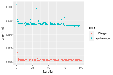
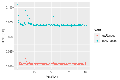 Table: Benchmarking of colRanges() and rowRanges() on double+10x10 data (original and transposed). The top panel shows times in milliseconds and the bottom panel shows relative times.
| expr | min | lq | mean | median | uq | max | |
|---|---|---|---|---|---|---|---|
| 1 | colRanges | 2.879 | 3.2545 | 4.14149 | 3.8460 | 4.7245 | 17.094 |
| 2 | rowRanges | 2.863 | 3.4115 | 4.64551 | 4.7015 | 4.9960 | 18.058 |
| expr | min | lq | mean | median | uq | max | |
|---|---|---|---|---|---|---|---|
| 1 | colRanges | 1.0000000 | 1.000000 | 1.0000 | 1.000000 | 1.000000 | 1.000000 |
| 2 | rowRanges | 0.9944425 | 1.048241 | 1.1217 | 1.222439 | 1.057466 | 1.056394 |
Figure: Benchmarking of colRanges() and rowRanges() on double+10x10 data (original and transposed). Outliers are displayed as crosses. Times are in milliseconds.
100x100 double matrix
> X <- data[["100x100"]]
> gc()
           used  (Mb) gc trigger  (Mb) max used  (Mb)
Ncells  5290540 282.6    7916910 422.9  7916910 422.9
Vcells 10213810  78.0   33191153 253.3 53339345 407.0
> colStats <- microbenchmark(colRanges = colRanges(X, na.rm = FALSE), `apply+range` = apply(X, MARGIN = 2L,
+     FUN = range, na.rm = FALSE), unit = "ms")
> X <- t(X)
> gc()
           used  (Mb) gc trigger  (Mb) max used  (Mb)
Ncells  5290534 282.6    7916910 422.9  7916910 422.9
Vcells 10223853  78.1   33191153 253.3 53339345 407.0
> rowStats <- microbenchmark(rowRanges = rowRanges(X, na.rm = FALSE), `apply+range` = apply(X, MARGIN = 1L,
+     FUN = range, na.rm = FALSE), unit = "ms")
Table: Benchmarking of colRanges() and apply+range() on double+100x100 data. The top panel shows times in milliseconds and the bottom panel shows relative times.
| expr | min | lq | mean | median | uq | max | |
|---|---|---|---|---|---|---|---|
| 1 | colRanges | 0.023408 | 0.0258655 | 0.0287942 | 0.0273385 | 0.0300845 | 0.058754 |
| 2 | apply+range | 0.384650 | 0.4139755 | 0.4521284 | 0.4273005 | 0.4828200 | 0.670138 |
| expr | min | lq | mean | median | uq | max | |
|---|---|---|---|---|---|---|---|
| 1 | colRanges | 1.00000 | 1.00000 | 1.00000 | 1.00000 | 1.0000 | 1.00000 |
| 2 | apply+range | 16.43242 | 16.00493 | 15.70205 | 15.62999 | 16.0488 | 11.40583 |
Table: Benchmarking of rowRanges() and apply+range() on double+100x100 data (transposed). The top panel shows times in milliseconds and the bottom panel shows relative times.
| expr | min | lq | mean | median | uq | max | |
|---|---|---|---|---|---|---|---|
| 1 | rowRanges | 0.031904 | 0.0350040 | 0.0384628 | 0.036666 | 0.0398435 | 0.061222 |
| 2 | apply+range | 0.385608 | 0.4120555 | 0.4509709 | 0.430714 | 0.4840040 | 0.687707 |
| expr | min | lq | mean | median | uq | max | |
|---|---|---|---|---|---|---|---|
| 1 | rowRanges | 1.00000 | 1.00000 | 1.00000 | 1.00000 | 1.00000 | 1.000 |
| 2 | apply+range | 12.08651 | 11.77167 | 11.72487 | 11.74696 | 12.14763 | 11.233 |
Figure: Benchmarking of colRanges() and apply+range() on double+100x100 data as well as rowRanges() and apply+range() on the same data transposed. Outliers are displayed as crosses. Times are in milliseconds.

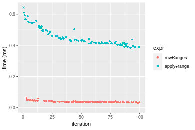 Table: Benchmarking of colRanges() and rowRanges() on double+100x100 data (original and transposed). The top panel shows times in milliseconds and the bottom panel shows relative times.
| expr | min | lq | mean | median | uq | max | |
|---|---|---|---|---|---|---|---|
| 1 | colRanges | 23.408 | 25.8655 | 28.79422 | 27.3385 | 30.0845 | 58.754 |
| 2 | rowRanges | 31.904 | 35.0040 | 38.46277 | 36.6660 | 39.8435 | 61.222 |
| expr | min | lq | mean | median | uq | max | |
|---|---|---|---|---|---|---|---|
| 1 | colRanges | 1.000000 | 1.000000 | 1.000000 | 1.000000 | 1.000000 | 1.000000 |
| 2 | rowRanges | 1.362953 | 1.353309 | 1.335781 | 1.341185 | 1.324386 | 1.042006 |
Figure: Benchmarking of colRanges() and rowRanges() on double+100x100 data (original and transposed). Outliers are displayed as crosses. Times are in milliseconds.
1000x10 double matrix
> X <- data[["1000x10"]]
> gc()
           used  (Mb) gc trigger  (Mb) max used  (Mb)
Ncells  5290730 282.6    7916910 422.9  7916910 422.9
Vcells 10214686  78.0   33191153 253.3 53339345 407.0
> colStats <- microbenchmark(colRanges = colRanges(X, na.rm = FALSE), `apply+range` = apply(X, MARGIN = 2L,
+     FUN = range, na.rm = FALSE), unit = "ms")
> X <- t(X)
> gc()
           used  (Mb) gc trigger  (Mb) max used  (Mb)
Ncells  5290724 282.6    7916910 422.9  7916910 422.9
Vcells 10224729  78.1   33191153 253.3 53339345 407.0
> rowStats <- microbenchmark(rowRanges = rowRanges(X, na.rm = FALSE), `apply+range` = apply(X, MARGIN = 1L,
+     FUN = range, na.rm = FALSE), unit = "ms")
Table: Benchmarking of colRanges() and apply+range() on double+1000x10 data. The top panel shows times in milliseconds and the bottom panel shows relative times.
| expr | min | lq | mean | median | uq | max | |
|---|---|---|---|---|---|---|---|
| 1 | colRanges | 0.020682 | 0.0233455 | 0.0255574 | 0.0247460 | 0.026293 | 0.052913 |
| 2 | apply+range | 0.174358 | 0.1907640 | 0.2073045 | 0.2074195 | 0.218942 | 0.319710 |
| expr | min | lq | mean | median | uq | max | |
|---|---|---|---|---|---|---|---|
| 1 | colRanges | 1.000000 | 1.000000 | 1.000000 | 1.000000 | 1.000000 | 1.000000 |
| 2 | apply+range | 8.430423 | 8.171339 | 8.111329 | 8.381941 | 8.327007 | 6.042183 |
Table: Benchmarking of rowRanges() and apply+range() on double+1000x10 data (transposed). The top panel shows times in milliseconds and the bottom panel shows relative times.
| expr | min | lq | mean | median | uq | max | |
|---|---|---|---|---|---|---|---|
| 1 | rowRanges | 0.030284 | 0.0338570 | 0.0409032 | 0.0367230 | 0.0414865 | 0.105211 |
| 2 | apply+range | 0.177154 | 0.1985895 | 0.2311509 | 0.2174635 | 0.2393390 | 0.692905 |
| expr | min | lq | mean | median | uq | max | |
|---|---|---|---|---|---|---|---|
| 1 | rowRanges | 1.000000 | 1.000000 | 1.000000 | 1.000000 | 1.000000 | 1.000000 |
| 2 | apply+range | 5.849756 | 5.865537 | 5.651173 | 5.921725 | 5.769082 | 6.585861 |
Figure: Benchmarking of colRanges() and apply+range() on double+1000x10 data as well as rowRanges() and apply+range() on the same data transposed. Outliers are displayed as crosses. Times are in milliseconds.
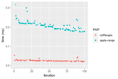
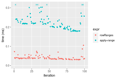 Table: Benchmarking of colRanges() and rowRanges() on double+1000x10 data (original and transposed). The top panel shows times in milliseconds and the bottom panel shows relative times.
| expr | min | lq | mean | median | uq | max | |
|---|---|---|---|---|---|---|---|
| 1 | colRanges | 20.682 | 23.3455 | 25.55740 | 24.746 | 26.2930 | 52.913 |
| 2 | rowRanges | 30.284 | 33.8570 | 40.90318 | 36.723 | 41.4865 | 105.211 |
| expr | min | lq | mean | median | uq | max | |
|---|---|---|---|---|---|---|---|
| 1 | colRanges | 1.000000 | 1.000000 | 1.000000 | 1.000000 | 1.000000 | 1.000000 |
| 2 | rowRanges | 1.464268 | 1.450258 | 1.600444 | 1.483997 | 1.577853 | 1.988377 |
Figure: Benchmarking of colRanges() and rowRanges() on double+1000x10 data (original and transposed). Outliers are displayed as crosses. Times are in milliseconds.
10x1000 double matrix
> X <- data[["10x1000"]]
> gc()
           used  (Mb) gc trigger  (Mb) max used  (Mb)
Ncells  5290918 282.6    7916910 422.9  7916910 422.9
Vcells 10215717  78.0   33191153 253.3 53339345 407.0
> colStats <- microbenchmark(colRanges = colRanges(X, na.rm = FALSE), `apply+range` = apply(X, MARGIN = 2L,
+     FUN = range, na.rm = FALSE), unit = "ms")
> X <- t(X)
> gc()
           used  (Mb) gc trigger  (Mb) max used  (Mb)
Ncells  5290912 282.6    7916910 422.9  7916910 422.9
Vcells 10225760  78.1   33191153 253.3 53339345 407.0
> rowStats <- microbenchmark(rowRanges = rowRanges(X, na.rm = FALSE), `apply+range` = apply(X, MARGIN = 1L,
+     FUN = range, na.rm = FALSE), unit = "ms")
Table: Benchmarking of colRanges() and apply+range() on double+10x1000 data. The top panel shows times in milliseconds and the bottom panel shows relative times.
| expr | min | lq | mean | median | uq | max | |
|---|---|---|---|---|---|---|---|
| 1 | colRanges | 0.051686 | 0.060895 | 0.0718143 | 0.0692865 | 0.079079 | 0.119015 |
| 2 | apply+range | 2.420775 | 2.699049 | 3.0359467 | 2.8332520 | 3.124196 | 9.275332 |
| expr | min | lq | mean | median | uq | max | |
|---|---|---|---|---|---|---|---|
| 1 | colRanges | 1.00000 | 1.000 | 1.00000 | 1.00000 | 1.00000 | 1.00000 |
| 2 | apply+range | 46.83618 | 44.323 | 42.27496 | 40.89183 | 39.50728 | 77.93414 |
Table: Benchmarking of rowRanges() and apply+range() on double+10x1000 data (transposed). The top panel shows times in milliseconds and the bottom panel shows relative times.
| expr | min | lq | mean | median | uq | max | |
|---|---|---|---|---|---|---|---|
| 1 | rowRanges | 0.051484 | 0.0540105 | 0.0623394 | 0.058000 | 0.067957 | 0.106699 |
| 2 | apply+range | 2.201806 | 2.3151420 | 2.5563392 | 2.441146 | 2.631711 | 8.012906 |
| expr | min | lq | mean | median | uq | max | |
|---|---|---|---|---|---|---|---|
| 1 | rowRanges | 1.0000 | 1.00000 | 1.00000 | 1.00000 | 1.00000 | 1.00000 |
| 2 | apply+range | 42.7668 | 42.86467 | 41.00682 | 42.08872 | 38.72612 | 75.09823 |
Figure: Benchmarking of colRanges() and apply+range() on double+10x1000 data as well as rowRanges() and apply+range() on the same data transposed. Outliers are displayed as crosses. Times are in milliseconds.
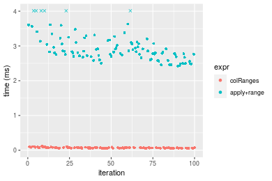
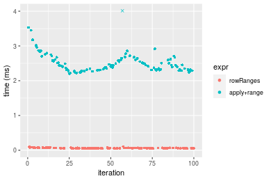 Table: Benchmarking of colRanges() and rowRanges() on double+10x1000 data (original and transposed). The top panel shows times in milliseconds and the bottom panel shows relative times.
| expr | min | lq | mean | median | uq | max | |
|---|---|---|---|---|---|---|---|
| 2 | rowRanges | 51.484 | 54.0105 | 62.33937 | 58.0000 | 67.957 | 106.699 |
| 1 | colRanges | 51.686 | 60.8950 | 71.81431 | 69.2865 | 79.079 | 119.015 |
| expr | min | lq | mean | median | uq | max | |
|---|---|---|---|---|---|---|---|
| 2 | rowRanges | 1.000000 | 1.000000 | 1.00000 | 1.000000 | 1.000000 | 1.000000 |
| 1 | colRanges | 1.003923 | 1.127466 | 1.15199 | 1.194595 | 1.163662 | 1.115428 |
Figure: Benchmarking of colRanges() and rowRanges() on double+10x1000 data (original and transposed). Outliers are displayed as crosses. Times are in milliseconds.
100x1000 double matrix
> X <- data[["100x1000"]]
> gc()
           used  (Mb) gc trigger  (Mb) max used  (Mb)
Ncells  5291114 282.6    7916910 422.9  7916910 422.9
Vcells 10215858  78.0   33191153 253.3 53339345 407.0
> colStats <- microbenchmark(colRanges = colRanges(X, na.rm = FALSE), `apply+range` = apply(X, MARGIN = 2L,
+     FUN = range, na.rm = FALSE), unit = "ms")
> X <- t(X)
> gc()
           used  (Mb) gc trigger  (Mb) max used  (Mb)
Ncells  5291096 282.6    7916910 422.9  7916910 422.9
Vcells 10315881  78.8   33191153 253.3 53339345 407.0
> rowStats <- microbenchmark(rowRanges = rowRanges(X, na.rm = FALSE), `apply+range` = apply(X, MARGIN = 1L,
+     FUN = range, na.rm = FALSE), unit = "ms")
Table: Benchmarking of colRanges() and apply+range() on double+100x1000 data. The top panel shows times in milliseconds and the bottom panel shows relative times.
| expr | min | lq | mean | median | uq | max | |
|---|---|---|---|---|---|---|---|
| 1 | colRanges | 0.207962 | 0.2318125 | 0.2615825 | 0.251070 | 0.2766675 | 0.474887 |
| 2 | apply+range | 3.020312 | 3.1727460 | 3.8239588 | 3.310179 | 3.8593650 | 24.960700 |
| expr | min | lq | mean | median | uq | max | |
|---|---|---|---|---|---|---|---|
| 1 | colRanges | 1.00000 | 1.00000 | 1.00000 | 1.00000 | 1.00000 | 1.00000 |
| 2 | apply+range | 14.52338 | 13.68669 | 14.61856 | 13.18429 | 13.94947 | 52.56135 |
Table: Benchmarking of rowRanges() and apply+range() on double+100x1000 data (transposed). The top panel shows times in milliseconds and the bottom panel shows relative times.
| expr | min | lq | mean | median | uq | max | |
|---|---|---|---|---|---|---|---|
| 1 | rowRanges | 0.265632 | 0.286015 | 0.318320 | 0.306714 | 0.342155 | 0.469355 |
| 2 | apply+range | 3.015830 | 3.304992 | 4.087795 | 3.660667 | 4.109141 | 23.201915 |
| expr | min | lq | mean | median | uq | max | |
|---|---|---|---|---|---|---|---|
| 1 | rowRanges | 1.00000 | 1.00000 | 1.00000 | 1.00000 | 1.00000 | 1.00000 |
| 2 | apply+range | 11.35341 | 11.55531 | 12.84178 | 11.93512 | 12.00959 | 49.43362 |
Figure: Benchmarking of colRanges() and apply+range() on double+100x1000 data as well as rowRanges() and apply+range() on the same data transposed. Outliers are displayed as crosses. Times are in milliseconds.
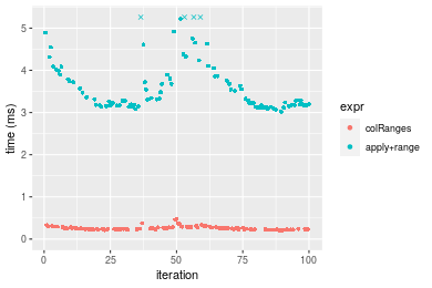
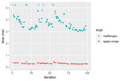 Table: Benchmarking of colRanges() and rowRanges() on double+100x1000 data (original and transposed). The top panel shows times in milliseconds and the bottom panel shows relative times.
| expr | min | lq | mean | median | uq | max | |
|---|---|---|---|---|---|---|---|
| 1 | colRanges | 207.962 | 231.8125 | 261.5825 | 251.070 | 276.6675 | 474.887 |
| 2 | rowRanges | 265.632 | 286.0150 | 318.3200 | 306.714 | 342.1550 | 469.355 |
| expr | min | lq | mean | median | uq | max | |
|---|---|---|---|---|---|---|---|
| 1 | colRanges | 1.00000 | 1.00000 | 1.000000 | 1.000000 | 1.000000 | 1.0000000 |
| 2 | rowRanges | 1.27731 | 1.23382 | 1.216901 | 1.221627 | 1.236701 | 0.9883509 |
Figure: Benchmarking of colRanges() and rowRanges() on double+100x1000 data (original and transposed). Outliers are displayed as crosses. Times are in milliseconds.
1000x100 double matrix
> X <- data[["1000x100"]]
> gc()
           used  (Mb) gc trigger  (Mb) max used  (Mb)
Ncells  5291306 282.6    7916910 422.9  7916910 422.9
Vcells 10217072  78.0   33191153 253.3 53339345 407.0
> colStats <- microbenchmark(colRanges = colRanges(X, na.rm = FALSE), `apply+range` = apply(X, MARGIN = 2L,
+     FUN = range, na.rm = FALSE), unit = "ms")
> X <- t(X)
> gc()
           used  (Mb) gc trigger  (Mb) max used  (Mb)
Ncells  5291288 282.6    7916910 422.9  7916910 422.9
Vcells 10317095  78.8   33191153 253.3 53339345 407.0
> rowStats <- microbenchmark(rowRanges = rowRanges(X, na.rm = FALSE), `apply+range` = apply(X, MARGIN = 1L,
+     FUN = range, na.rm = FALSE), unit = "ms")
Table: Benchmarking of colRanges() and apply+range() on double+1000x100 data. The top panel shows times in milliseconds and the bottom panel shows relative times.
| expr | min | lq | mean | median | uq | max | |
|---|---|---|---|---|---|---|---|
| 1 | colRanges | 0.142391 | 0.152734 | 0.1735739 | 0.167516 | 0.1864305 | 0.280665 |
| 2 | apply+range | 1.100118 | 1.188143 | 1.4283477 | 1.299945 | 1.4674575 | 9.004336 |
| expr | min | lq | mean | median | uq | max | |
|---|---|---|---|---|---|---|---|
| 1 | colRanges | 1.000000 | 1.000000 | 1.000000 | 1.000000 | 1.000000 | 1.00000 |
| 2 | apply+range | 7.726036 | 7.779162 | 8.229048 | 7.760121 | 7.871338 | 32.08215 |
Table: Benchmarking of rowRanges() and apply+range() on double+1000x100 data (transposed). The top panel shows times in milliseconds and the bottom panel shows relative times.
| expr | min | lq | mean | median | uq | max | |
|---|---|---|---|---|---|---|---|
| 1 | rowRanges | 0.219919 | 0.2248505 | 0.2570479 | 0.2453945 | 0.2789315 | 0.444242 |
| 2 | apply+range | 1.124972 | 1.1448900 | 1.4296463 | 1.2933755 | 1.4817175 | 8.798881 |
| expr | min | lq | mean | median | uq | max | |
|---|---|---|---|---|---|---|---|
| 1 | rowRanges | 1.000000 | 1.000000 | 1.00000 | 1.000000 | 1.00000 | 1.0000 |
| 2 | apply+range | 5.115392 | 5.091783 | 5.56179 | 5.270597 | 5.31212 | 19.8065 |
Figure: Benchmarking of colRanges() and apply+range() on double+1000x100 data as well as rowRanges() and apply+range() on the same data transposed. Outliers are displayed as crosses. Times are in milliseconds.
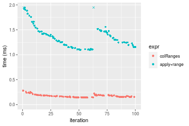
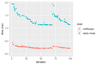 Table: Benchmarking of colRanges() and rowRanges() on double+1000x100 data (original and transposed). The top panel shows times in milliseconds and the bottom panel shows relative times.
| expr | min | lq | mean | median | uq | max | |
|---|---|---|---|---|---|---|---|
| 1 | colRanges | 142.391 | 152.7340 | 173.5739 | 167.5160 | 186.4305 | 280.665 |
| 2 | rowRanges | 219.919 | 224.8505 | 257.0479 | 245.3945 | 278.9315 | 444.242 |
| expr | min | lq | mean | median | uq | max | |
|---|---|---|---|---|---|---|---|
| 1 | colRanges | 1.000000 | 1.000000 | 1.000000 | 1.000000 | 1.000000 | 1.000000 |
| 2 | rowRanges | 1.544473 | 1.472171 | 1.480913 | 1.464902 | 1.496169 | 1.582819 |
Figure: Benchmarking of colRanges() and rowRanges() on double+1000x100 data (original and transposed). Outliers are displayed as crosses. Times are in milliseconds.
Appendix
Session information
R version 4.1.1 Patched (2021-08-10 r80727)
Platform: x86_64-pc-linux-gnu (64-bit)
Running under: Ubuntu 18.04.5 LTS

Matrix products: default
BLAS:   /home/hb/software/R-devel/R-4-1-branch/lib/R/lib/libRblas.so
LAPACK: /home/hb/software/R-devel/R-4-1-branch/lib/R/lib/libRlapack.so

locale:
 [1] LC_CTYPE=en_US.UTF-8       LC_NUMERIC=C
 [3] LC_TIME=en_US.UTF-8        LC_COLLATE=en_US.UTF-8
 [5] LC_MONETARY=en_US.UTF-8    LC_MESSAGES=en_US.UTF-8
 [7] LC_PAPER=en_US.UTF-8       LC_NAME=C
 [9] LC_ADDRESS=C               LC_TELEPHONE=C
[11] LC_MEASUREMENT=en_US.UTF-8 LC_IDENTIFICATION=C

attached base packages:
[1] stats     graphics  grDevices utils     datasets  methods   base

other attached packages:
[1] microbenchmark_1.4-7   matrixStats_0.60.0     ggplot2_3.3.5
[4] knitr_1.33             R.devices_2.17.0       R.utils_2.10.1
[7] R.oo_1.24.0            R.methodsS3_1.8.1-9001 history_0.0.1-9000

loaded via a namespace (and not attached):
 [1] Biobase_2.52.0          httr_1.4.2              splines_4.1.1
 [4] bit64_4.0.5             network_1.17.1          assertthat_0.2.1
 [7] highr_0.9               stats4_4.1.1            blob_1.2.2
[10] GenomeInfoDbData_1.2.6  robustbase_0.93-8       pillar_1.6.2
[13] RSQLite_2.2.8           lattice_0.20-44         glue_1.4.2
[16] digest_0.6.27           XVector_0.32.0          colorspace_2.0-2
[19] Matrix_1.3-4            XML_3.99-0.7            pkgconfig_2.0.3
[22] zlibbioc_1.38.0         genefilter_1.74.0       purrr_0.3.4
[25] ergm_4.1.2              xtable_1.8-4            scales_1.1.1
[28] tibble_3.1.4            annotate_1.70.0         KEGGREST_1.32.0
[31] farver_2.1.0            generics_0.1.0          IRanges_2.26.0
[34] ellipsis_0.3.2          cachem_1.0.6            withr_2.4.2
[37] BiocGenerics_0.38.0     mime_0.11               survival_3.2-13
[40] magrittr_2.0.1          crayon_1.4.1            statnet.common_4.5.0
[43] memoise_2.0.0           laeken_0.5.1            fansi_0.5.0
[46] R.cache_0.15.0          MASS_7.3-54             R.rsp_0.44.0
[49] progressr_0.8.0         tools_4.1.1             lifecycle_1.0.0
[52] S4Vectors_0.30.0        trust_0.1-8             munsell_0.5.0
[55] tabby_0.0.1-9001        AnnotationDbi_1.54.1    Biostrings_2.60.2
[58] compiler_4.1.1          GenomeInfoDb_1.28.1     rlang_0.4.11
[61] grid_4.1.1              RCurl_1.98-1.4          cwhmisc_6.6
[64] rstudioapi_0.13         rappdirs_0.3.3          startup_0.15.0
[67] labeling_0.4.2          bitops_1.0-7            base64enc_0.1-3
[70] boot_1.3-28             gtable_0.3.0            DBI_1.1.1
[73] markdown_1.1            R6_2.5.1                lpSolveAPI_5.5.2.0-17.7
[76] rle_0.9.2               dplyr_1.0.7             fastmap_1.1.0
[79] bit_4.0.4               utf8_1.2.2              parallel_4.1.1
[82] Rcpp_1.0.7              vctrs_0.3.8             png_0.1-7
[85] DEoptimR_1.0-9          tidyselect_1.1.1        xfun_0.25
[88] coda_0.19-4
Total processing time was 27.25 secs.
Reproducibility
To reproduce this report, do:
html <- matrixStats:::benchmark('colRanges')
Copyright Henrik Bengtsson. Last updated on 2021-08-25 22:27:48 (+0200 UTC). Powered by RSP.