matrixStats.benchmarks

---

colQuantiles() and rowQuantiles() benchmarks

This report benchmark the performance of colQuantiles() and rowQuantiles() against alternative methods.

Alternative methods

• apply() + quantile()

Data

> rmatrix <- function(nrow, ncol, mode = c("logical", "double", "integer", "index"), range = c(-100, 
+     +100), na_prob = 0) {
+     mode <- match.arg(mode)
+     n <- nrow * ncol
+     if (mode == "logical") {
+         x <- sample(c(FALSE, TRUE), size = n, replace = TRUE)
+     }     else if (mode == "index") {
+         x <- seq_len(n)
+         mode <- "integer"
+     }     else {
+         x <- runif(n, min = range[1], max = range[2])
+     }
+     storage.mode(x) <- mode
+     if (na_prob > 0) 
+         x[sample(n, size = na_prob * n)] <- NA
+     dim(x) <- c(nrow, ncol)
+     x
+ }
> rmatrices <- function(scale = 10, seed = 1, ...) {
+     set.seed(seed)
+     data <- list()
+     data[[1]] <- rmatrix(nrow = scale * 1, ncol = scale * 1, ...)
+     data[[2]] <- rmatrix(nrow = scale * 10, ncol = scale * 10, ...)
+     data[[3]] <- rmatrix(nrow = scale * 100, ncol = scale * 1, ...)
+     data[[4]] <- t(data[[3]])
+     data[[5]] <- rmatrix(nrow = scale * 10, ncol = scale * 100, ...)
+     data[[6]] <- t(data[[5]])
+     names(data) <- sapply(data, FUN = function(x) paste(dim(x), collapse = "x"))
+     data
+ }
> data <- rmatrices(mode = "double")

Results

10x10 matrix

> X <- data[["10x10"]]
> gc()
           used  (Mb) gc trigger  (Mb) max used  (Mb)
Ncells  5283699 282.2    7916910 422.9  7916910 422.9
Vcells 10537175  80.4   33191153 253.3 53339345 407.0
> probs <- seq(from = 0, to = 1, by = 0.25)
> colStats <- microbenchmark(colQuantiles = colQuantiles(X, probs = probs, na.rm = FALSE), `apply+quantile` = apply(X, 
+     MARGIN = 2L, FUN = quantile, probs = probs, na.rm = FALSE), unit = "ms")
> X <- t(X)
> gc()
           used  (Mb) gc trigger  (Mb) max used  (Mb)
Ncells  5283507 282.2    7916910 422.9  7916910 422.9
Vcells 10536953  80.4   33191153 253.3 53339345 407.0
> rowStats <- microbenchmark(rowQuantiles = rowQuantiles(X, probs = probs, na.rm = FALSE), `apply+quantile` = apply(X, 
+     MARGIN = 1L, FUN = quantile, probs = probs, na.rm = FALSE), unit = "ms")

Table: Benchmarking of colQuantiles() and apply+quantile() on 10x10 data. The top panel shows times in milliseconds and the bottom panel shows relative times.

	expr	min	lq	mean	median	uq	max
1	colQuantiles	0.302906	0.329424	0.3677154	0.359026	0.3966375	0.540448
2	apply+quantile	1.364473	1.438469	1.5741078	1.511068	1.7432090	2.199361

	expr	min	lq	mean	median	uq	max
1	colQuantiles	1.000000	1.000000	1.000000	1.000000	1.000000	1.000000
2	apply+quantile	4.504609	4.366619	4.280778	4.208797	4.394968	4.069515

Table: Benchmarking of rowQuantiles() and apply+quantile() on 10x10 data (transposed). The top panel shows times in milliseconds and the bottom panel shows relative times.

	expr	min	lq	mean	median	uq	max
1	rowQuantiles	0.239440	0.258194	0.3004935	0.2638625	0.3232105	0.561646
2	apply+quantile	1.063889	1.103623	1.2585152	1.1329855	1.3459045	2.063830

	expr	min	lq	mean	median	uq	max
1	rowQuantiles	1.000000	1.000000	1.000000	1.000000	1.000000	1.00000
2	apply+quantile	4.443238	4.274394	4.188162	4.293848	4.164173	3.67461

Figure: Benchmarking of colQuantiles() and apply+quantile() on 10x10 data as well as rowQuantiles() and apply+quantile() on the same data transposed. Outliers are displayed as crosses. Times are in milliseconds.

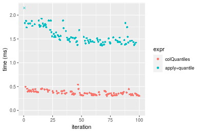
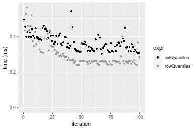
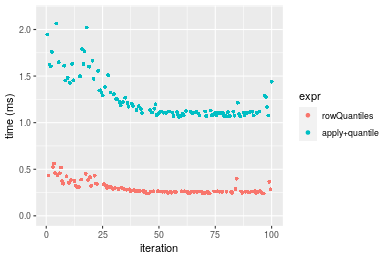Table: Benchmarking of colQuantiles() and rowQuantiles() on 10x10 data (original and transposed). The top panel shows times in milliseconds and the bottom panel shows relative times.

	expr	min	lq	mean	median	uq	max
2	rowQuantiles	239.440	258.194	300.4935	263.8625	323.2105	561.646
1	colQuantiles	302.906	329.424	367.7154	359.0260	396.6375	540.448

	expr	min	lq	mean	median	uq	max
2	rowQuantiles	1.00000	1.000000	1.000000	1.000000	1.00000	1.0000000
1	colQuantiles	1.26506	1.275878	1.223705	1.360656	1.22718	0.9622574

Figure: Benchmarking of colQuantiles() and rowQuantiles() on 10x10 data (original and transposed). Outliers are displayed as crosses. Times are in milliseconds.

100x100 matrix

> X <- data[["100x100"]]
> gc()
           used  (Mb) gc trigger  (Mb) max used  (Mb)
Ncells  5282073 282.1    7916910 422.9  7916910 422.9
Vcells 10153396  77.5   33191153 253.3 53339345 407.0
> probs <- seq(from = 0, to = 1, by = 0.25)
> colStats <- microbenchmark(colQuantiles = colQuantiles(X, probs = probs, na.rm = FALSE), `apply+quantile` = apply(X, 
+     MARGIN = 2L, FUN = quantile, probs = probs, na.rm = FALSE), unit = "ms")
> X <- t(X)
> gc()
           used  (Mb) gc trigger  (Mb) max used  (Mb)
Ncells  5282061 282.1    7916910 422.9  7916910 422.9
Vcells 10163429  77.6   33191153 253.3 53339345 407.0
> rowStats <- microbenchmark(rowQuantiles = rowQuantiles(X, probs = probs, na.rm = FALSE), `apply+quantile` = apply(X, 
+     MARGIN = 1L, FUN = quantile, probs = probs, na.rm = FALSE), unit = "ms")

Table: Benchmarking of colQuantiles() and apply+quantile() on 100x100 data. The top panel shows times in milliseconds and the bottom panel shows relative times.

	expr	min	lq	mean	median	uq	max
1	colQuantiles	1.843692	1.90874	2.24609	1.97988	2.13335	8.8629
2	apply+quantile	10.674418	10.90321	15.60727	11.17651	12.21271	381.8870

	expr	min	lq	mean	median	uq	max
1	colQuantiles	1.000000	1.000000	1.000000	1.000000	1.000000	1.00000
2	apply+quantile	5.789697	5.712257	6.948642	5.645043	5.724664	43.08827

Table: Benchmarking of rowQuantiles() and apply+quantile() on 100x100 data (transposed). The top panel shows times in milliseconds and the bottom panel shows relative times.

	expr	min	lq	mean	median	uq	max
1	rowQuantiles	1.901765	1.98259	2.19478	2.039334	2.332585	3.054295
2	apply+quantile	10.722477	11.10321	12.93694	11.629099	14.161271	24.969997

	expr	min	lq	mean	median	uq	max
1	rowQuantiles	1.000000	1.000000	1.000000	1.000000	1.000000	1.000000
2	apply+quantile	5.638171	5.600357	5.894414	5.702402	6.071062	8.175372

Figure: Benchmarking of colQuantiles() and apply+quantile() on 100x100 data as well as rowQuantiles() and apply+quantile() on the same data transposed. Outliers are displayed as crosses. Times are in milliseconds.

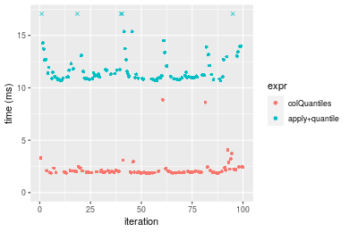
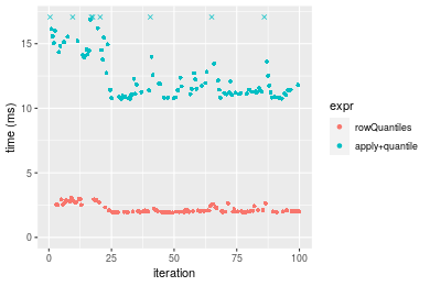Table: Benchmarking of colQuantiles() and rowQuantiles() on 100x100 data (original and transposed). The top panel shows times in milliseconds and the bottom panel shows relative times.

	expr	min	lq	mean	median	uq	max
1	colQuantiles	1.843692	1.90874	2.24609	1.979880	2.133350	8.862900
2	rowQuantiles	1.901765	1.98259	2.19478	2.039334	2.332585	3.054295

	expr	min	lq	mean	median	uq	max
1	colQuantiles	1.000000	1.000000	1.0000000	1.000000	1.000000	1.0000000
2	rowQuantiles	1.031498	1.038691	0.9771561	1.030029	1.093391	0.3446158

Figure: Benchmarking of colQuantiles() and rowQuantiles() on 100x100 data (original and transposed). Outliers are displayed as crosses. Times are in milliseconds.

1000x10 matrix

> X <- data[["1000x10"]]
> gc()
           used  (Mb) gc trigger  (Mb) max used  (Mb)
Ncells  5282815 282.2    7916910 422.9  7916910 422.9
Vcells 10156922  77.5   33191153 253.3 53339345 407.0
> probs <- seq(from = 0, to = 1, by = 0.25)
> colStats <- microbenchmark(colQuantiles = colQuantiles(X, probs = probs, na.rm = FALSE), `apply+quantile` = apply(X, 
+     MARGIN = 2L, FUN = quantile, probs = probs, na.rm = FALSE), unit = "ms")
> X <- t(X)
> gc()
           used  (Mb) gc trigger  (Mb) max used  (Mb)
Ncells  5282791 282.2    7916910 422.9  7916910 422.9
Vcells 10166935  77.6   33191153 253.3 53339345 407.0
> rowStats <- microbenchmark(rowQuantiles = rowQuantiles(X, probs = probs, na.rm = FALSE), `apply+quantile` = apply(X, 
+     MARGIN = 1L, FUN = quantile, probs = probs, na.rm = FALSE), unit = "ms")

Table: Benchmarking of colQuantiles() and apply+quantile() on 1000x10 data. The top panel shows times in milliseconds and the bottom panel shows relative times.

	expr	min	lq	mean	median	uq	max
1	colQuantiles	0.590347	0.6104945	0.681985	0.6246515	0.678449	1.248694
2	apply+quantile	1.476754	1.5267405	1.687743	1.5651400	1.762205	2.788720

	expr	min	lq	mean	median	uq	max
1	colQuantiles	1.000000	1.000000	1.000000	1.000000	1.000000	1.000000
2	apply+quantile	2.501502	2.500826	2.474751	2.505621	2.597402	2.233309

Table: Benchmarking of rowQuantiles() and apply+quantile() on 1000x10 data (transposed). The top panel shows times in milliseconds and the bottom panel shows relative times.

	expr	min	lq	mean	median	uq	max
1	rowQuantiles	0.626120	0.6527315	0.736542	0.691613	0.807727	1.219093
2	apply+quantile	1.494004	1.5361655	1.707736	1.597339	1.789035	2.667647

	expr	min	lq	mean	median	uq	max
1	rowQuantiles	1.000000	1.000000	1.000000	1.000000	1.000000	1.000000
2	apply+quantile	2.386131	2.353442	2.318586	2.309586	2.214901	2.188223

Figure: Benchmarking of colQuantiles() and apply+quantile() on 1000x10 data as well as rowQuantiles() and apply+quantile() on the same data transposed. Outliers are displayed as crosses. Times are in milliseconds.

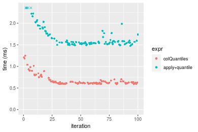
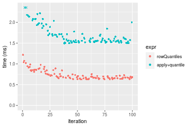Table: Benchmarking of colQuantiles() and rowQuantiles() on 1000x10 data (original and transposed). The top panel shows times in milliseconds and the bottom panel shows relative times.

	expr	min	lq	mean	median	uq	max
1	colQuantiles	590.347	610.4945	681.985	624.6515	678.449	1248.694
2	rowQuantiles	626.120	652.7315	736.542	691.6130	807.727	1219.093

	expr	min	lq	mean	median	uq	max
1	colQuantiles	1.000000	1.000000	1.000000	1.000000	1.000000	1.0000000
2	rowQuantiles	1.060597	1.069185	1.079997	1.107198	1.190549	0.9762944

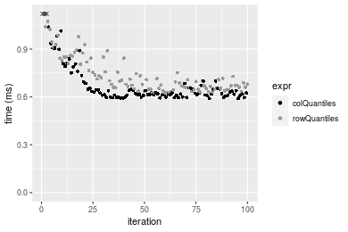
Figure: Benchmarking of colQuantiles() and rowQuantiles() on 1000x10 data (original and transposed). Outliers are displayed as crosses. Times are in milliseconds.

10x1000 matrix

> X <- data[["10x1000"]]
> gc()
           used  (Mb) gc trigger  (Mb) max used  (Mb)
Ncells  5282991 282.2    7916910 422.9  7916910 422.9
Vcells 10157622  77.5   33191153 253.3 53339345 407.0
> probs <- seq(from = 0, to = 1, by = 0.25)
> colStats <- microbenchmark(colQuantiles = colQuantiles(X, probs = probs, na.rm = FALSE), `apply+quantile` = apply(X, 
+     MARGIN = 2L, FUN = quantile, probs = probs, na.rm = FALSE), unit = "ms")
> X <- t(X)
> gc()
           used  (Mb) gc trigger  (Mb) max used  (Mb)
Ncells  5282979 282.2    7916910 422.9  7916910 422.9
Vcells 10167655  77.6   33191153 253.3 53339345 407.0
> rowStats <- microbenchmark(rowQuantiles = rowQuantiles(X, probs = probs, na.rm = FALSE), `apply+quantile` = apply(X, 
+     MARGIN = 1L, FUN = quantile, probs = probs, na.rm = FALSE), unit = "ms")

Table: Benchmarking of colQuantiles() and apply+quantile() on 10x1000 data. The top panel shows times in milliseconds and the bottom panel shows relative times.

	expr	min	lq	mean	median	uq	max
1	colQuantiles	13.55287	14.01786	15.7543	14.57951	16.36505	26.8499
2	apply+quantile	100.83011	104.24423	112.1036	110.51778	117.83936	145.3915

	expr	min	lq	mean	median	uq	max
1	colQuantiles	1.00000	1.000000	1.000000	1.000000	1.000000	1.000000
2	apply+quantile	7.43976	7.436527	7.115746	7.580347	7.200672	5.414975

Table: Benchmarking of rowQuantiles() and apply+quantile() on 10x1000 data (transposed). The top panel shows times in milliseconds and the bottom panel shows relative times.

	expr	min	lq	mean	median	uq	max
1	rowQuantiles	13.58450	13.81358	15.58997	14.30125	15.59021	32.9124
2	apply+quantile	99.82761	104.50799	114.91728	112.48729	121.21521	178.8486

	expr	min	lq	mean	median	uq	max
1	rowQuantiles	1.00000	1.000000	1.000000	1.000000	1.000000	1.00000
2	apply+quantile	7.34864	7.565596	7.371232	7.865559	7.775085	5.43408

Figure: Benchmarking of colQuantiles() and apply+quantile() on 10x1000 data as well as rowQuantiles() and apply+quantile() on the same data transposed. Outliers are displayed as crosses. Times are in milliseconds.

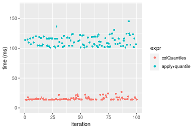
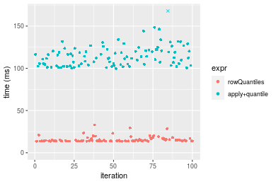Table: Benchmarking of colQuantiles() and rowQuantiles() on 10x1000 data (original and transposed). The top panel shows times in milliseconds and the bottom panel shows relative times.

	expr	min	lq	mean	median	uq	max
2	rowQuantiles	13.58450	13.81358	15.58997	14.30125	15.59021	32.9124
1	colQuantiles	13.55287	14.01786	15.75430	14.57951	16.36505	26.8499

	expr	min	lq	mean	median	uq	max
2	rowQuantiles	1.0000000	1.000000	1.000000	1.000000	1.0000	1.0000000
1	colQuantiles	0.9976717	1.014788	1.010541	1.019458	1.0497	0.8157989

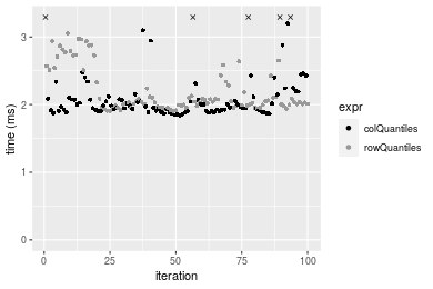
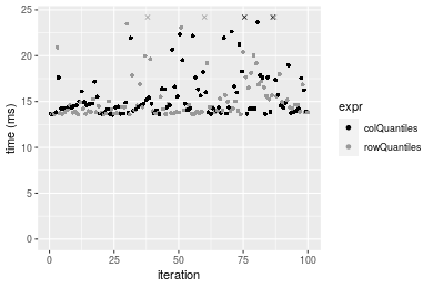
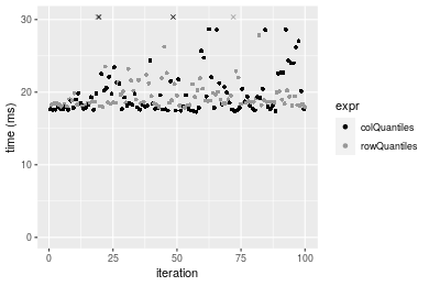
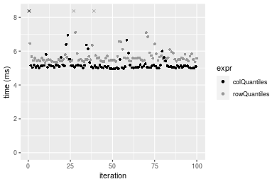
Figure: Benchmarking of colQuantiles() and rowQuantiles() on 10x1000 data (original and transposed). Outliers are displayed as crosses. Times are in milliseconds.

100x1000 matrix

> X <- data[["100x1000"]]
> gc()
           used  (Mb) gc trigger  (Mb) max used  (Mb)
Ncells  5283181 282.2    7916910 422.9  7916910 422.9
Vcells 10158119  77.6   33191153 253.3 53339345 407.0
> probs <- seq(from = 0, to = 1, by = 0.25)
> colStats <- microbenchmark(colQuantiles = colQuantiles(X, probs = probs, na.rm = FALSE), `apply+quantile` = apply(X, 
+     MARGIN = 2L, FUN = quantile, probs = probs, na.rm = FALSE), unit = "ms")
> X <- t(X)
> gc()
           used  (Mb) gc trigger  (Mb) max used  (Mb)
Ncells  5283163 282.2    7916910 422.9  7916910 422.9
Vcells 10258142  78.3   33191153 253.3 53339345 407.0
> rowStats <- microbenchmark(rowQuantiles = rowQuantiles(X, probs = probs, na.rm = FALSE), `apply+quantile` = apply(X, 
+     MARGIN = 1L, FUN = quantile, probs = probs, na.rm = FALSE), unit = "ms")

Table: Benchmarking of colQuantiles() and apply+quantile() on 100x1000 data. The top panel shows times in milliseconds and the bottom panel shows relative times.

	expr	min	lq	mean	median	uq	max
1	colQuantiles	17.29224	17.73178	23.86813	18.47384	21.20117	412.5931
2	apply+quantile	106.29891	109.58439	123.38824	121.01874	130.89134	196.2455

	expr	min	lq	mean	median	uq	max
1	colQuantiles	1.000000	1.000000	1.000000	1.000000	1.00000	1.0000000
2	apply+quantile	6.147205	6.180113	5.169581	6.550816	6.17378	0.4756392

Table: Benchmarking of rowQuantiles() and apply+quantile() on 100x1000 data (transposed). The top panel shows times in milliseconds and the bottom panel shows relative times.

	expr	min	lq	mean	median	uq	max
1	rowQuantiles	17.89716	18.4045	19.64489	18.70136	20.01506	31.27969
2	apply+quantile	106.93395	111.9668	123.09826	121.39408	131.45883	161.34232

	expr	min	lq	mean	median	uq	max
1	rowQuantiles	1.000000	1.000000	1.000000	1.000000	1.000000	1.000000
2	apply+quantile	5.974913	6.083664	6.266172	6.491189	6.567997	5.158054

Figure: Benchmarking of colQuantiles() and apply+quantile() on 100x1000 data as well as rowQuantiles() and apply+quantile() on the same data transposed. Outliers are displayed as crosses. Times are in milliseconds.

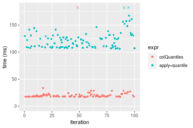
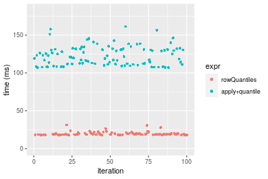Table: Benchmarking of colQuantiles() and rowQuantiles() on 100x1000 data (original and transposed). The top panel shows times in milliseconds and the bottom panel shows relative times.

	expr	min	lq	mean	median	uq	max
1	colQuantiles	17.29224	17.73178	23.86813	18.47384	21.20117	412.59314
2	rowQuantiles	17.89716	18.40450	19.64489	18.70136	20.01506	31.27969

	expr	min	lq	mean	median	uq	max
1	colQuantiles	1.000000	1.000000	1.0000000	1.000000	1.0000000	1.0000000
2	rowQuantiles	1.034982	1.037939	0.8230594	1.012316	0.9440544	0.0758124

Figure: Benchmarking of colQuantiles() and rowQuantiles() on 100x1000 data (original and transposed). Outliers are displayed as crosses. Times are in milliseconds.

1000x100 matrix

> X <- data[["1000x100"]]
> gc()
           used  (Mb) gc trigger  (Mb) max used  (Mb)
Ncells  5283373 282.2    7916910 422.9  7916910 422.9
Vcells 10158745  77.6   33191153 253.3 53339345 407.0
> probs <- seq(from = 0, to = 1, by = 0.25)
> colStats <- microbenchmark(colQuantiles = colQuantiles(X, probs = probs, na.rm = FALSE), `apply+quantile` = apply(X, 
+     MARGIN = 2L, FUN = quantile, probs = probs, na.rm = FALSE), unit = "ms")
> X <- t(X)
> gc()
           used  (Mb) gc trigger  (Mb) max used  (Mb)
Ncells  5283355 282.2    7916910 422.9  7916910 422.9
Vcells 10258768  78.3   33191153 253.3 53339345 407.0
> rowStats <- microbenchmark(rowQuantiles = rowQuantiles(X, probs = probs, na.rm = FALSE), `apply+quantile` = apply(X, 
+     MARGIN = 1L, FUN = quantile, probs = probs, na.rm = FALSE), unit = "ms")

Table: Benchmarking of colQuantiles() and apply+quantile() on 1000x100 data. The top panel shows times in milliseconds and the bottom panel shows relative times.

	expr	min	lq	mean	median	uq	max
1	colQuantiles	4.951451	5.02867	5.23471	5.110415	5.16578	8.446151
2	apply+quantile	14.330868	14.50606	15.34585	14.602870	14.90682	25.848297

	expr	min	lq	mean	median	uq	max
1	colQuantiles	1.000000	1.000000	1.000000	1.000000	1.000000	1.000000
2	apply+quantile	2.894276	2.884672	2.931556	2.857473	2.885687	3.060364

Table: Benchmarking of rowQuantiles() and apply+quantile() on 1000x100 data (transposed). The top panel shows times in milliseconds and the bottom panel shows relative times.

	expr	min	lq	mean	median	uq	max
1	rowQuantiles	5.324899	5.445932	5.764332	5.531068	5.691759	14.66775
2	apply+quantile	14.449878	14.704087	15.582007	14.877622	15.320830	26.38245

	expr	min	lq	mean	median	uq	max
1	rowQuantiles	1.000000	1.000000	1.000000	1.000000	1.000000	1.00000
2	apply+quantile	2.713644	2.700013	2.703177	2.689828	2.691756	1.79867

Figure: Benchmarking of colQuantiles() and apply+quantile() on 1000x100 data as well as rowQuantiles() and apply+quantile() on the same data transposed. Outliers are displayed as crosses. Times are in milliseconds.

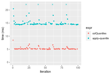
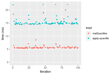Table: Benchmarking of colQuantiles() and rowQuantiles() on 1000x100 data (original and transposed). The top panel shows times in milliseconds and the bottom panel shows relative times.

	expr	min	lq	mean	median	uq	max
1	colQuantiles	4.951451	5.028670	5.234710	5.110415	5.165780	8.446151
2	rowQuantiles	5.324899	5.445932	5.764332	5.531068	5.691759	14.667752

	expr	min	lq	mean	median	uq	max
1	colQuantiles	1.000000	1.000000	1.000000	1.000000	1.00000	1.00000
2	rowQuantiles	1.075422	1.082977	1.101175	1.082313	1.10182	1.73662

Figure: Benchmarking of colQuantiles() and rowQuantiles() on 1000x100 data (original and transposed). Outliers are displayed as crosses. Times are in milliseconds.

Appendix

Session information

R version 4.1.1 Patched (2021-08-10 r80727)
Platform: x86_64-pc-linux-gnu (64-bit)
Running under: Ubuntu 18.04.5 LTS

Matrix products: default
BLAS:   /home/hb/software/R-devel/R-4-1-branch/lib/R/lib/libRblas.so
LAPACK: /home/hb/software/R-devel/R-4-1-branch/lib/R/lib/libRlapack.so

locale:
 [1] LC_CTYPE=en_US.UTF-8       LC_NUMERIC=C              
 [3] LC_TIME=en_US.UTF-8        LC_COLLATE=en_US.UTF-8    
 [5] LC_MONETARY=en_US.UTF-8    LC_MESSAGES=en_US.UTF-8   
 [7] LC_PAPER=en_US.UTF-8       LC_NAME=C                 
 [9] LC_ADDRESS=C               LC_TELEPHONE=C            
[11] LC_MEASUREMENT=en_US.UTF-8 LC_IDENTIFICATION=C       

attached base packages:
[1] stats     graphics  grDevices utils     datasets  methods   base     

other attached packages:
[1] microbenchmark_1.4-7   matrixStats_0.60.0     ggplot2_3.3.5         
[4] knitr_1.33             R.devices_2.17.0       R.utils_2.10.1        
[7] R.oo_1.24.0            R.methodsS3_1.8.1-9001 history_0.0.1-9000    

loaded via a namespace (and not attached):
 [1] Biobase_2.52.0          httr_1.4.2              splines_4.1.1          
 [4] bit64_4.0.5             network_1.17.1          assertthat_0.2.1       
 [7] highr_0.9               stats4_4.1.1            blob_1.2.2             
[10] GenomeInfoDbData_1.2.6  robustbase_0.93-8       pillar_1.6.2           
[13] RSQLite_2.2.8           lattice_0.20-44         glue_1.4.2             
[16] digest_0.6.27           XVector_0.32.0          colorspace_2.0-2       
[19] Matrix_1.3-4            XML_3.99-0.7            pkgconfig_2.0.3        
[22] zlibbioc_1.38.0         genefilter_1.74.0       purrr_0.3.4            
[25] ergm_4.1.2              xtable_1.8-4            scales_1.1.1           
[28] tibble_3.1.4            annotate_1.70.0         KEGGREST_1.32.0        
[31] farver_2.1.0            generics_0.1.0          IRanges_2.26.0         
[34] ellipsis_0.3.2          cachem_1.0.6            withr_2.4.2            
[37] BiocGenerics_0.38.0     mime_0.11               survival_3.2-13        
[40] magrittr_2.0.1          crayon_1.4.1            statnet.common_4.5.0   
[43] memoise_2.0.0           laeken_0.5.1            fansi_0.5.0            
[46] R.cache_0.15.0          MASS_7.3-54             R.rsp_0.44.0           
[49] progressr_0.8.0         tools_4.1.1             lifecycle_1.0.0        
[52] S4Vectors_0.30.0        trust_0.1-8             munsell_0.5.0          
[55] tabby_0.0.1-9001        AnnotationDbi_1.54.1    Biostrings_2.60.2      
[58] compiler_4.1.1          GenomeInfoDb_1.28.1     rlang_0.4.11           
[61] grid_4.1.1              RCurl_1.98-1.4          cwhmisc_6.6            
[64] rstudioapi_0.13         rappdirs_0.3.3          startup_0.15.0         
[67] labeling_0.4.2          bitops_1.0-7            base64enc_0.1-3        
[70] boot_1.3-28             gtable_0.3.0            DBI_1.1.1              
[73] markdown_1.1            R6_2.5.1                lpSolveAPI_5.5.2.0-17.7
[76] rle_0.9.2               dplyr_1.0.7             fastmap_1.1.0          
[79] bit_4.0.4               utf8_1.2.2              parallel_4.1.1         
[82] Rcpp_1.0.7              vctrs_0.3.8             png_0.1-7              
[85] DEoptimR_1.0-9          tidyselect_1.1.1        xfun_0.25              
[88] coda_0.19-4            

Total processing time was 1.25 mins.

Reproducibility

To reproduce this report, do:

html <- matrixStats:::benchmark('colQuantiles')

---

Copyright Henrik Bengtsson. Last updated on 2021-08-25 22:26:54 (+0200 UTC). Powered by RSP.