f <- function(x) 2*x
y <- f(1)
z <- f(3)Introduction to Parallel Processing in R using Futureverse - Easier than Ever Before
Henrik Bengtsson
University of California, San Francisco
R Foundation, R Consortium, Bioconductor
@HenrikBengtsson



useR! 2026, Warsaw, Poland (July 6, 2026)
About me
- Used R since September 2000
- MSc Computer Science, PhD Mathematical Statistics
- Applied research in genomics and bioinformatics
- Always had a need to speed up analyses and share worldwide
- Creator of the future ecosystem (“futureverse”) - anno 2015
- Best thing in R: The R community! People nerding out on R
How about you?
Q1. How many R conferences have you attended before?
- my first!
- my second
- three or more
Q2. For how long have you used R?
- < 1 year
- 1-2 years
- 3-5 years
- > 5 years
Q3. Have you used parallelization in R before?
- never
- tried, but failed
- yes, some
- yes, a lot
Q4. What R parallelization methods have you used?
Q5. Reason for attending this parallelization tutorial?
Q6. What operating system do you use today?
- Windows
- macOS
- Linux
Q7. How do you run R today?
- in the terminal
- in RStudio
- in Positron
- in Rgui
- …?
Why do we parallelize code?
Parallel & distributed processing can be used to:
- speed up processing (wall time)
- lower memory footprint (per machine)
- avoid data transfers (compute where data lives)
- other reasons, e.g. asynchronous UI
How do we parallelize code?
We may choose to parallelize on:
- our personal laptop or work desktop computer (single user)
- a shared powerful computer (multiple users)
- across many computers, e.g. in the office or in the cloud
- high-performance compute (HPC) cluster (multiple users) with a job scheduler, e.g. Slurm, Son of Grid Engine (SGE), TORQUE/PBS, …
Your turn: Install and load ‘futureverse’
Step 1: Install packages
Step 2: Make sure everything is up-to-date
Step 3: Verify it works
Your turn: Measuring processing times
We can measure the processing time of our code using system.time().
Define a slow function
Running times for different input lengths
Your turn: Measuring processing times using in-house toc()
We can measure the processing time of our code using tic()/toc() from the futureverse package:
Measure running times via progress reporting
All you need to remember is progressify()
Your turn: Introducing progressify
We can get a progress bar by piping our calls to progressify().
Default output (using the built-in utils::txtProgressBar()):
> ys <- lapply(1:10, slow_sqrt) |> progressify()
|=============================        | 80%
Progress bar is erased on completion.
Your turn: Styled progress reporting
We can customize the style of the progress bar using the cli package.
Output:
> ys <- lapply(1:10, slow_sqrt) |> progressify()
■■■■■■■■■■■■■■■■■■■■■■■■■         80% | ETA:  1s
Progress bar is erased on completion.
Your turn: Make some noise!
We can combine multiple progress handlers:
Output:
> ys <- lapply(1:10, slow_sqrt) |> progressify()
■■■■■■■■■■■■■■■■■■■■■■■■■         80% | ETA:  1s
with ♫♪♬♫ … ♬♫
Progress bar is erased on completion.
Your turn: Keep the progress output when done
By default, progress bars are erased on completion. This feature can be disabled, but to keep things simple, we will use a special “tutorial” handler today:
Output:
> ys <- lapply(1:10, slow_sqrt) |> progressify()
[ 5s] | [============================] 100% [10/10] (ETA:  0s)
>
Progress bar remains beyond completion.
Your turn: Keep all progress updates
By default, the progress bars are cleared at each update, and also at the very end. Because of this, we will use a special “tutorial” handler for this workshop:
Output:
> ys <- lapply(1:10, slow_sqrt) |> progressify()
[ 0s] - [-----------------------------]   0% [0/10] (ETA:  ?s)
[ 1s] \ [==>--------------------------]  10% [1/10] (ETA:  5s)
[ 1s] | [=====>-----------------------]  20% [2/10] (ETA:  4s)
[ 2s] / [========>--------------------]  30% [3/10] (ETA:  4s)
[ 2s] - [===========>-----------------]  40% [4/10] (ETA:  3s)
[ 3s] \ [==============>--------------]  50% [5/10] (ETA:  3s)
[ 3s] | [=================>-----------]  60% [6/10] (ETA:  2s)
[ 4s] / [====================>--------]  70% [7/10] (ETA:  2s)
[ 4s] - [=======================>-----]  80% [8/10] (ETA:  1s)
[ 5s] \ [==========================>--]  90% [9/10] (ETA:  1s)
[ 5s] | [============================] 100% [10/10] (ETA:  0s)
>
Progress output remains beyond completion.
R: A Functional Programming Language

R is a functional programming language
Mathematics:
\[ \begin{aligned} f(x) &= 2 \cdot x \\ y &= f(1) \\ z &= f(3) \end{aligned} \]
R:
A function has code, arguments, and a value
A function has:
- code, e.g.
2*x - arguments (“parameters”), e.g.
x - a value
A function can take multiple arguments
A function has:
- code, e.g.
b*x - arguments (“parameters”), e.g.
xandb - a value
When we call the function:
R evaluates the code with the values of arguments x (= 4) and b (= 2), returns the value, and assigns the value to variable y.
Arguments can have default values
When we call the function:
R evaluates the code with the value of argument x (= 4), the default value of b (= 2), returns the value, and assigns the value to variable y.
Summation
\[ h(\mathbf{x}) = \sum_{i=1}^{n} x_i ; \mathbf{x} = (x_1, x_2, \ldots, x_n) \\ \]
Summation - emulate slowness
\[ h(\mathbf{x}) = \sum_{i=1}^{n} x_i ; \mathbf{x} = (x_1, x_2, \ldots, x_n) \\ \]
Summation can be done in parts
\[ h(\mathbf{x}) = \sum_{i=1}^{n} x_i \]
\[ \phantom{h(\mathbf{x})} = \sum_{i=1}^{k} x_i + \sum_{i=k+1}^{n} x_i \\ \]
\[ \phantom{h(\mathbf{x})} = h(\mathbf{x}_{1:k}) + h(\mathbf{x}_{(k+1):n}) \]
Summation can be done in parts
\[ \begin{aligned} h(\mathbf{x}) &= \sum_{i=1}^{n} x_i \\ \mathbf{x} &= (1, 2, \ldots, 10) \end{aligned} \]
\[ y = h(\mathbf{x}) \]
\[ \begin{aligned} a &= h(\mathbf{x}_{1:5}) \\ b &= h(\mathbf{x}_{6:10}) \\ y &= a + b \end{aligned} \]
\[ y = 55 \]
Summation of parts can be done in any order
\[ \begin{aligned} a &= h(\mathbf{x}_{1:5}) \\ b &= h(\mathbf{x}_{6:10}) \\ y &= a + b \end{aligned} \]
\[ y = 55 \]
Concurrent summation of parts
\[ \text{concurrently} \left\{\begin{matrix} a = h(\mathbf{x}_{1:5}) \\ b = h(\mathbf{x}_{6:10}) \\ \end{matrix}\right. \\ \hspace{10ex} y = a + b \]
How can we calculate \(a\) and \(b\) concurrently in R?
a and b take 5 seconds each => everything takes ~5 seconds
Package ‘future’ adds support for concurrent programming in R
%<-%is called the future-assignment operator
Your turn: Setup
Step 3: Implement \(h()\) as above, but call it slow_sum()
Your turn: Verify
Step 4: Test slow_sum()
Create \(x = (1, 2, ..., 10)\) in R
Call
y <- slow_sum(x)and confirm it takes 10 secondsCall
a <- slow_sum(x[1:5])and confirm it takes 5 secondsSame for
b <- slow_sum(x[6:10])
Your turn: Our very first concurrent evaluation of R code
Step 5: Sum parts concurrently
Confirm correct result
Confirm that it finishes in 5 seconds - use
tic()/toc()How long does each line take? - use
tic()/toc()Something else?
Note on y <- a + b |> toc()
Note that:
is the same as:
which is not what we wanted, i.e.
Concurrent Programming in R
Future … what?
- A future is an abstraction for a value that will be available later
- The state of a future is either unresolved or resolved
- The value is the result of an evaluated expression
References
Friedman & Wise (1976, 1977), Hibbard (1976), Baker & Hewitt (1977)
Your turn: future() and value()
Verify result
Verify total run time
Verify run time per line
Functions
Functions and Futures
Futureverse - A Friendly, Unifying Parallelization Framework in R
- “Write once, run anywhere” - a simple unified API
- 100% cross-platform - easy to install
- Works with any type of parallel backend
- Very well tested, lots of CPU mileage
11 years, used by 1,600 packages, top-0.6% downloaded
Low friction:
- Automatically exports global variables
- Automatically relays output, messages, and warnings
- Proper parallel random number generation (RNG)
- … and much more
Globals automatically found (99.5% worry-free)
Static-code inspection by walking the abstract syntax tree (AST):
=> globals identified and exported to the worker:
slow_sum()- a function (also searched recursively)x- a numeric vector of length 100
Apply the same function over and over
For-loop:
Apply the same function over and over
Base R:
Apply the same function over and over
Plyr:
Foreach:
Take-home: lapply(), map(), llply(), foreach() all the same
Pipes: Syntactic sugar to spice it up
Base R:
is identical to
R can’t tell the difference! (e.g. try with lobstr::ast(...))
Your turn: Draw an Owl

Your turn: Start with a for-loop
Task: Create a function ys <- parallel_map(xs, slow_sqrt)
Combine the idea of:
with:
to make a “concurrent” for-loop.
Hint: You need two for-loops - one for future() and one for value()
Your turn: Concurrent for-loop to concurrent map
Coffee Break (30 mins)
Your turn: Create parallel_map()
Building blocks:
Your turn: Benchmark map() vs parallel_map()
Compare how fast:
is compared to:
- Use
system.time()ortic()/toc()
Why is value(fs) preferred over lapply(fs, value)?
lapply(fs, value) resolves futures sequentially:
- No early stopping: If the third future fails,
lapply()still blocks waiting for the first and second futures to finish. - Orphaned workers: If a future fails, the remaining running futures are left running on the workers, wasting resources.
Vectorized value(fs) is aware of all futures:
- Early stopping: If any future fails, times out, or its worker crashes,
value()immediately throws the error. - Automatic cancellation: Outstanding futures are sent a termination signal, instantly freeing up the workers.
ys <- parallel_map(xs, slow_sqrt)
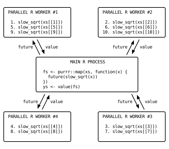

Good job! You’ve learned a lot!
- The concept of “futures” was invented in 1975 (sic!)
- Basic building blocks
future()andvalue()are very powerful - You can create richer parallelization functions from these, e.g.
parallel_map()
Now, let’s simplify our lives …
All you need to remember is futurize()
Futureverse allows you to stick to your favorite coding style
Parallel alternatives to traditional, sequential functions:
future.apply and furrr?
futurize()is new since January 2026- future.apply, furrr, and doFuture are now only used in the background
Futures can be resolved anywhere!
Our ys <- map(xs, slow_sqrt) |> futurize() can be resolved on lots of different backends - it doesn’t matter where!
On the current machine
plan(sequential)
sequentially (default)
plan(multisession)
plan(multisession, workers=4)
in parallel via background R workers
plan(future.mirai::mirai_multisession)
plan(future.mirai::mirai_multisession, workers=4)
in parallel via future.mirai; low latency
plan(future.callr::callr)
plan(future.callr::callr, workers=4)
in parallel via future.callr; all memory is returned as each future is resolved
Futures can be resolved anywhere!
On other machines
plan(cluster, workers=c("n1", "m2.uni.edu", "vm.cloud.org"))
distributed on other local or remote computers
plan(future.mirai::mirai)
distributed via future.mirai daemon queue
On high-performance compute (HPC) cluster
In parallel on HPC job schedulers for long-running tasks with higher latency.
HPC processing: future.batchtools
Making progress in parallel . . .
All you need to remember is futurize() + progressify()
Progress reporting + Parallel processing
You can combine progressify() and futurize() to get progress reporting in parallel:
Output:
ys <- lapply(xs, slow_sqrt) |> progressify() |> futurize()
■■■■■■■■■■■■■■■■■■■■■■■■■         80% | ETA:  1s
Progress is reported in a near-live fashion.
Your turn: Try different backends
Sequential:
Built-in multisession:
Add-on mirai-based multisession:
Your turn: Benchmark with different number of workers
Run:
Then benchmark with:
- Try to call
plan()without arguments
Your turn: Benchmark different backends
Run:
Then benchmark with:
Messages, Warnings, and Errors
Some functions have side effects
What type of results may this function produce?
Your turn: Messages, warnings, and errors with futures
Your turn: Errors terminate calls
Your turn: Errors terminate parallelized calls
Business as usual but in parallel
Things we haven’t talked about
Random number generation (RNG) in parallel processing
Random numbers need extra care when tasks run in parallel.
Using rnorm() without declaring it:
Warning message:
UNRELIABLE VALUE: Future (...) unexpectedly generated random numbers
without specifying argument 'seed'. There is a risk that those random
numbers are not statistically sound and the overall results might be
invalid. To fix this, specify 'seed = TRUE'. ...
Declaring parallel-safe RNG with seed = TRUE:
Why it matters:
- Workers can share or overlap the same random stream => duplicated or correlated draws
- Results may change with the number of workers and the backend => not reproducible
seed = TRUEuses the parallel-safe L’Ecuyer-CMRG generator to give each task its own independent, reproducible stream
When parallelization does not help
Parallelization adds overhead - it is not always a win.
Parallelization can be slower when:
- Tasks are too small - per-task overhead (launch, serialize, transfer) exceeds the actual work
- Data is large - copying inputs and outputs to and from workers dominates
- The bottleneck is not the CPU - disk-, network-, or memory-bandwidth-bound work does not speed up
- The code is already vectorized - e.g.
sqrt(xs)beats any parallel map
Rules of thumb
- Parallelize the slow, coarse chunks, not the tiny fast ones
- Group many small tasks into fewer larger ones (chunking)
- Measure - use
tic()/toc(), don’t assume
Not everything can travel to a worker
Some objects are tied to your current R session and cannot be exported to a worker:
- Database connections (DBI), open file or socket connections
- External pointers - xgboost, torch, keras/tensorflow, Rcpp
- reticulate Python objects
Error: Detected a non-exportable reference in the globals:
'con' of class 'SQLiteConnection' uses an external pointer
Enable early detection with options(future.globals.onReference = "error").
Parallelizing select domain-specific calls
library(futurize); plan(multisession, workers = 8)
library(progressify); handlers("tutorial")

# Simulate dataset
n <- 5000
data <- data.frame(y = rbinom(n, 1, 0.5), x1 = rnorm(n), x2 = rnorm(n))

# Fit logistic regression
fit_glm <- function(data, indices) {
  coef(glm(y ~ x1 + x2, data = data[indices, ], family = binomial))
}

# Bootstrap
b <- boot::boot(data, statistic = fit_glm, R = 1000) |> progressify() |> futurize()- I’m giving a talk on futurize on Wednesday at 14:00
The same futurize() works across your stats packages
Popular statistics & ML packages support futurize() - no new API to learn:
# Bootstrap ({boot})
boot::boot(data, statistic, R = 1000)         |> futurize()

# Cross-validation ({glmnet})
glmnet::cv.glmnet(x, y)                       |> futurize()

# Model tuning ({caret})
caret::train(y ~ ., data = d, method = "rf")  |> futurize()

# Additive models ({mgcv})
mgcv::bam(y ~ s(x1) + s(x2), data = d)        |> futurize()

# Mixed-model bootstrap ({lme4})
lme4::bootMer(fit, statistic, nsim = 1000)    |> futurize()
Your existing call, plus one pipe - it runs on whatever backend plan() you chose.
Under the hood: futurize() is a transpiler
futurize() doesn’t parallelize your call directly - it rewrites (“transpiles”) it into the equivalent Futureverse call, then evaluates that.
Pass eval = FALSE to see the generated code instead of running it:
The same holds for domain-specific packages - inspect what boot generates:
local({
    cl <- do.call(future::makeClusterFuture, args = list(seed = FALSE,
        globals = TRUE, stdout = TRUE, conditions = "condition",
        label = "fz:boot::boot"))
    oopts <- options(future.ClusterFuture.clusterEvalQ = "ignore")
    on.exit(options(oopts))
    boot::boot(data, statistic, R = 1000, parallel = "snow",
        ncpus = 2L, cl = cl)
})
Each supported package has its own transpiler mapping the sequential call to a parallel backend.
Nested parallelization with some care
- “Structured concurrency” -
Futureverse protects against over-parallelization


Sequential
processing
Parallelization
with 4 workers
Nested parallelization
with 5 workers each
running 3 parallel tasks
Cheat sheet (1/2): choose a backend & parallelize
library(futurize)

## 1. Choose WHERE to run (once)
plan(sequential)                        # default - no parallelism
plan(multisession, workers = 4)         # background R workers
plan(cluster, workers = c("n1", "n2"))  # other machines

## 2. Parallelize - just add a pipe
ys <- lapply(xs, fcn)             |> futurize()
ys <- purrr::map(xs, fcn)         |> futurize()
ys <- foreach(x = xs) %do% fcn(x) |> futurize()
Cheat sheet (2/2): progress, RNG & building blocks
The future is bright!
Coming: Efficient memory handling
- Shared memory support is on the horizon:
- Powered by the upcoming mori package
- Credit to the old Bioconductor SharedObject package (which is very similar)
- Shared memory only works on parallel workers running on the same machine
- I aim to make it fully automatic, so you will not have to do anything
- When released, all existing code will automatically see an improvement
Coming: Resource management
- Declarative Resource API:
Avoid Resource Waste:
- Conservative: prevent impossible runs - early stopping
- Scheduling: avoid running out of memory, HPC job scheduling, …
Monitor Resources:
- Track and monitor resource usage (e.g. CPU, GPU, memory, runtime) during execution
- Predict Resources: (possibly also)
- Model resource needs over time, e.g. runtime and memory
- Predict resource needs on the input, e.g. suggest specifications, better progress ETA
Thank you - Enjoy useR! 💜
- It’s easy to get started - just try
futurize() - Website: https://www.futureverse.org/
- Blog: https://www.futureverse.org/blog.html
- Support: https://github.com/orgs/futureverse/discussions
- Exciting features on the roadmap
- I love bug reports, feedback and ideas
Appendix
foreach() is not a for loop!

We must never think of foreach() as a for-loop
The name foreach() tricks us into believing it’s a for-loop
!=
Repeat after me: foreach() is not a for-loop! 🎶

foreach() is just like lapply() …
This does not work, because the <- assignment is done inside a function
… and just like map() …
This does not work, because the <- assignment is done inside a function